Transformers and Attention
Attention
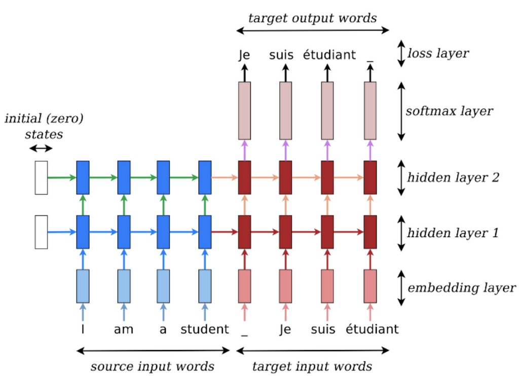
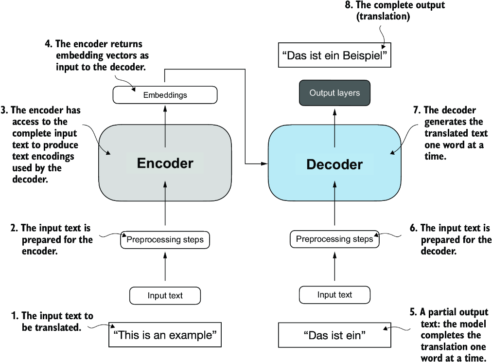
Seq2Seq Models with encoder-decoder architectures looked to encode the entire context into a singular vector that got passed to each decoder step, which led to bottlenecks, inefficiencies, etc
Attention, as an embedding concept, is what separates static embeddings from dynamic embeddings - they allow word embeddings to be updated, aka attended to, by the contextual words surrounding them
Transformers as an architecture helped to make attention a parallelizable function, ultimately allowing for context to spread in a way that no longer bottlenecked infromation into a context vector, and allowed for large scale SIMD type of parallel processing
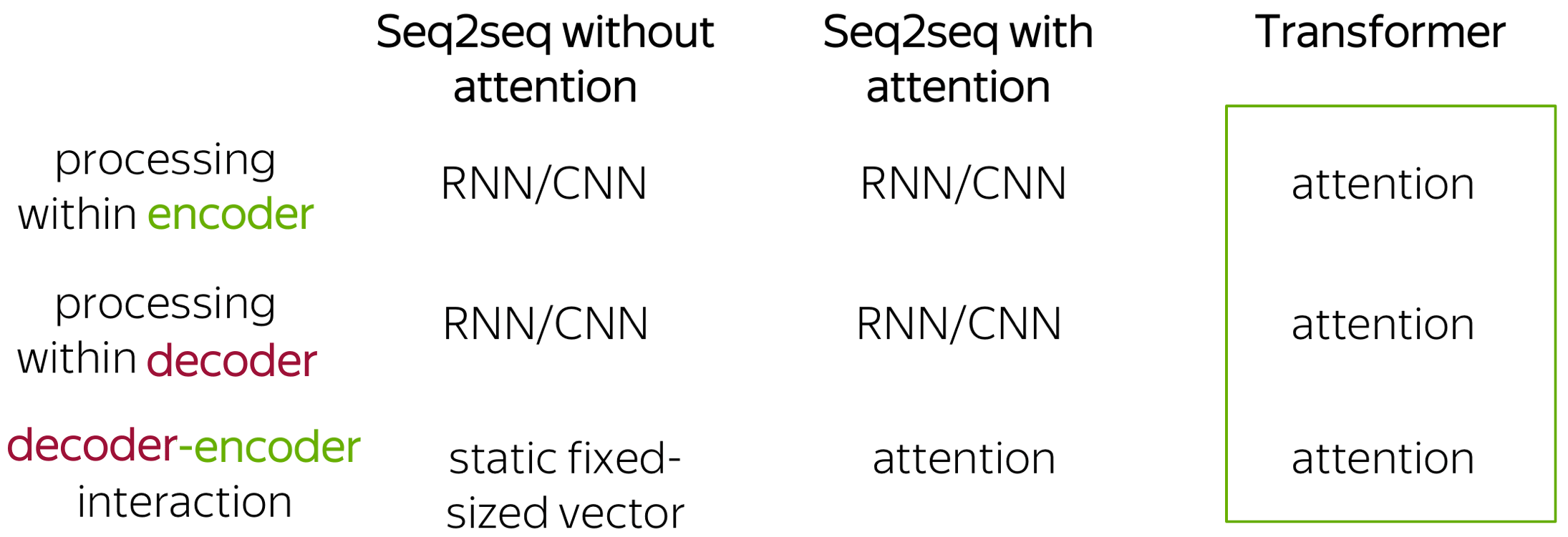
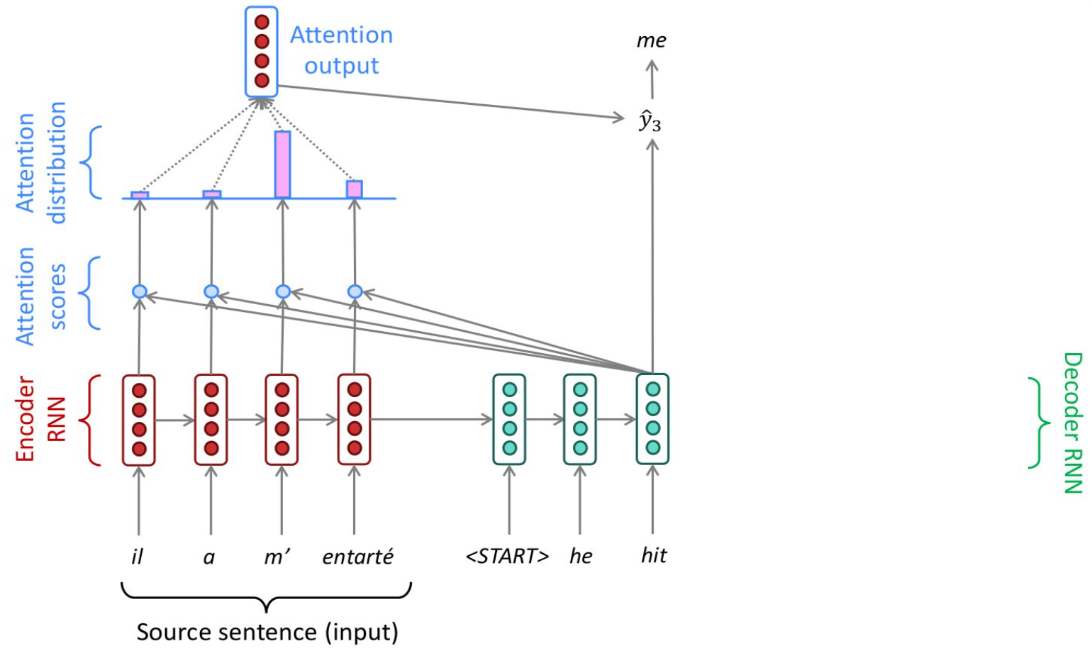
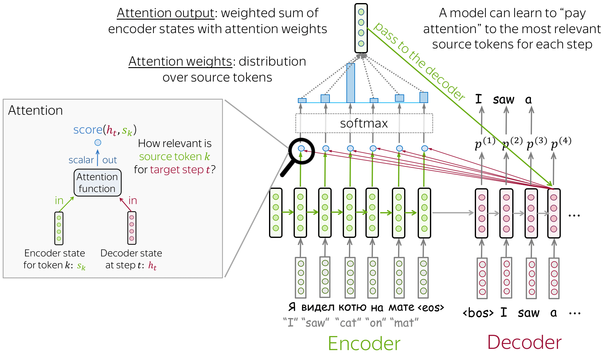
NLP Seq2Seq Tasks like next word prediction, and translation where using the surrounding context of the word was one of the major breakthroughs in achieving better Seq2Seq results. Attention helps to fix the bottleneck problem in RNN encoder (and RNN encoder-decoder) models - Due to their design, the encoding of the source sentence is a single vector representation (context vector). The problem is that this state must compress all information about the source sentence in a single vector and this is commonly referred to as the bottleneck problem. There was a desire to not "squish" everything into one single context vector, and instead to utilize the input embeddings dynamically when decoding, and to utilize the context on the fly - this is known as align and translate jointly
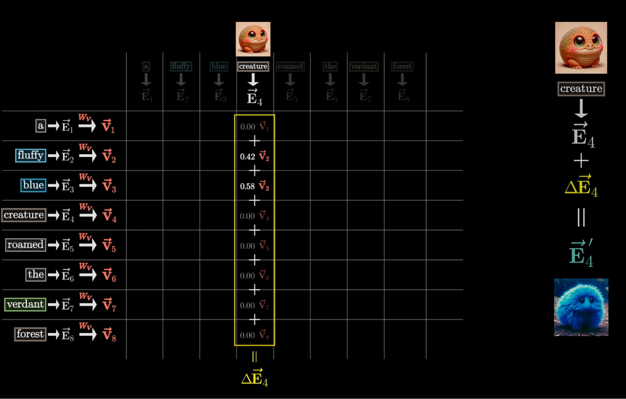
The embedding for "bank" is always the same embedding in the metric space in static scenario's like Word2Vec, but by attending to it with Attention, you can change it's position! It's as simple as that, so at the end of attending to the vector, the vector for bank in river bank may point in a completely different direction than the vector for bank in bank vault - just because of how the other words add or detract from it geometrically in its metric space. Bank + having river in sentence moves vector in matrix space closer to a sand dune, where Bank + teller in sentence moves it closer to a financial worker
How is this done? Attention mechanisms in our DNN models. There are multiple forms of Attention - most useful / used are Self Attention, Encoder-Decoder Attention, and Masked Self Attention - each of them help to attend to a current query word / position based on it's surroundings. A single head of this Attention mechanism would only update certain "relationships", or attended to geometric shifts, but mutliple different Attention mechanisms might be able to learn a dynamic range of relationships
In the days before Attention, there would be Encoders that take input sentence and write it to a fixed size embedding layer, and then a separately trained Decoder that would take the embedding and output a new sentence - this architecture for Seq2Seq tasks is fine for short sequences, but degrades with longer sequences you try to "stuff into" a fixed size embedding layer
Therefore, Attention helps us to remove this fixed size constraint between encoders and decoders, but attention does no more than weighted averaging, and so without neural network layer functions it's strictly weighted averaging. Transformers help change this and add in non-linear layers
All of these Attention mechanisms are tunable matrices of weights - they are learned and updated through the model training process, and it's why you need to "bring along the model" during inference...otherwise you can't use the Attention!
Below shows an example of how an embedding like creature would change based on surrounding context
Or showcasing how adjective / adverb positions are different between languages
Keys, Queries, and Values Intuition
Lots of the excerpts here are from the D2L AI Blog on Attention
Consider a K:V database, it may have tuples such as ('Luke', 'Sprangers'), ('Donald', 'Duck'), ('Jeff', 'Bezos'), ..., ('Puke', 'Skywalker') with first and last names - if you wanted to query the database, we'd simply query based on a key like Database.get('Luke') and it would return Sprangers
If you allow for approximate matches, you might get ['Sprangers', 'Skywalker']
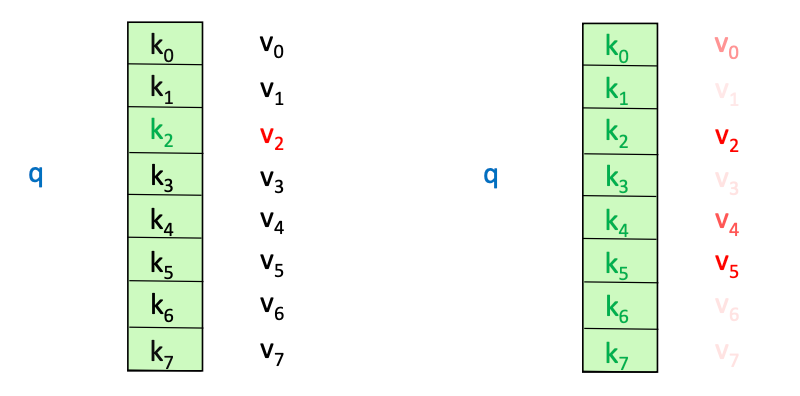
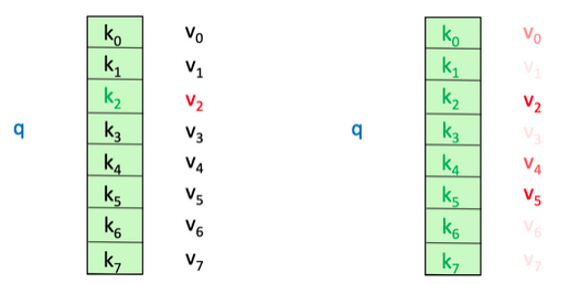
Therefore, our Queries and our Keys have a relationship! They can be exact, or they can be similar (Luke and Puke are similar), and based on those similarities, you may or may not want to return a Value. Thinking of self-attention as an approximate hash table eases understanding its intuition. To look up a value, queries are compared against keys in a table. In a hash table, which is shown on the left side of image below, there is exactly one key-value pair for each query (hash). In contrast, in self-attention, each key is matched to varying degrees by each query. Thus, a sum of values weighted by the query-key match is returned
What if you wanted to return a portion of the Value, based on how similar our Query was to our Key? Luke and Luke are 1:1, so you fully return Sprangers, but Luke and Puke are slightly different, so what if you returned something like intersect / total * Value, or 75% of the Value?
Luke and Puke have letters as the same, so you can return of Skywalker!
This is the exact idea of Attention -
This attention can be read as "for every key / value pair , compare the key and the value with , and based on how similar they are return that much of the value. The total sum of all those values is the value you will return"
Therefore, you can mimic an exact lookup if you define our as a Kronecker Delta:
This means we'll return the list of all values that match Luke, which is just 1
Another example would be if
D = [
   ([1, 0], 4),
   ([1, 1], 6),
   ([0, 1], 6)
]
And our Query is [0.5, 0] - if you compare that to all of our Keys, we'd see distance([0.5, 0] - [1, 0]) = 0.5 and distance([0.5, 0] - [1, 1]) = - 0.5 so you would have 0.5 * 4 + -0.5 * 6 = -1 would be our answer!
So these comparisons of Queries and Keys results in some weight, and typically you will compare our Query to every Key, and the resulting set you will stuff through a Softmax function to get weights that sum to 1
To ensure weights are non-negative, you can use exponentiation
This is exactly what will come through in most attention calculations!
Parameters
In discussions below, we'll use these parameters to talk through time and memory complexities, along with architectures and layers
The input is usually a sequence of size , which has a number of tokens , and each of these tokens will go through a static embedding layer to create input embeddings of size (typically 128). After this, the embeddings of size will all go through multiple layers of normalization, dropout, and self-attention to produce output hidden states. These output hidden states are of size (typically 512), and there would still be final states, one for each input. These final hidden states are labeled
- Parameters:
- layers / encoder blocks
- is the size of the hidden states
- 256 is typical size of hidden state dimension
- is the encoder hidden size
- is the decoder hidden size
- is the alignment MLP hidden size
- attention heads per layer
- Typically 6 attention heads
- represents the input embedding dimension
- 128 is typical embedding dimension
- represents the final hidden vector (of size ) of our
[CLS]token (i.e. our "final" hidden layer for our sentence) - as the final hidden state for a specific input token
- is our positional encoding which represents the learned positional embedding for our token in it's specific sentence of any size
- is our segment encoding which represents the learned positional embedding for our token in either segment sentence A or B
- In our inference time examples for embeddings most people just fill it with
0'sor1'sdepending on which sentence it's apart of
- In our inference time examples for embeddings most people just fill it with
Bahdanau RNN Attention
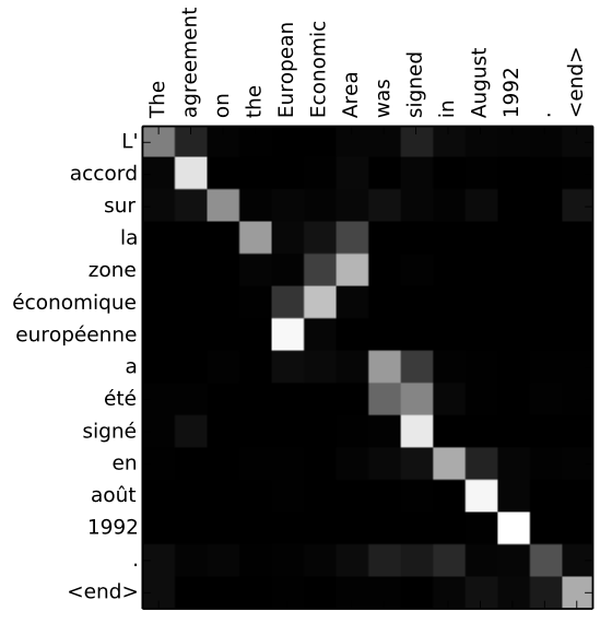
Things first started off with Bahdanau Style RNN Attention via Neural Machine Translation by Jointly Learning to Align and Translate (2014)
This paper discusses how most architectures of the time have a 2 pronged setup:
- An encoder to take the source sentence into a fixed length vector
- In most scenario's there's an encoder-per-language
- A decoder to take that fixed length vector, and output a translated sentence
- There's also typically a decoder-per-language as well
- Therefore, for every language there's an encoder-decoder pair which is jointly trained to maximize the probability of correct translation
- Why is this bad?
- Requires every translation problem to be "squished" into the same fixed-length vector
- Examples cited of how the performance of this encoder-decoder architecture deteriorates rapidly as the length of input sentence increases
- Proposal in this paper:
- "you introduce an extension of the encoder-decoder model which learns to align and translate jointly"
- This means it sets up (aligns) and decodes (translates) on the fly over the entire sentence, and not just all at once
- "Each time the proposed model generates a word in a translation, it (soft-)searches for a set of positions in a source sentence where the most relevant information is concentrated
- This means it uses some sort of comparison (later seen as attention) to figure out what words are most relevant in the translation
- The model then predicts a target word based on the context vectors associated with these source positions and all previously generated target words
- The model predicst the next word based on attention of this word and input sentence + previously generated words
- This was a breakthrough in attention, but apparently was proposed here earlier!
- "you introduce an extension of the encoder-decoder model which learns to align and translate jointly"
- Altogether, this architecture looks to break away from encoding the entire input into one single vector by encoding the input into a sequence of vectors which it uses adaptively while decoding
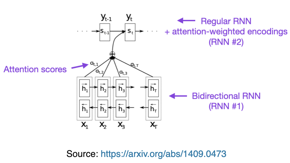
- The bottom portion is an encoder which receives source sentence as input
- The top part is a decoder, which outputs the translated sentence
Encoder RNN Attention
- Input: A sequence of vectors
- Encoder Hidden States:
- is some non-linear function
- This will take the current input embedding, and the output of the last recurrence
- These are bi-directional
-
- Concatenation!
- It is formalized that is the hidden state of the encoder at time
- Encoder Hidden States:
- These
- They live entirely in the encoder block
- They are fixed once the input is encoded
Decoder RNN Attention
Decoder is often trained to predict the next word given the context vector and all the previously predicted words
Our translation can be defined as which is just the sequence of words output so far!
It does this by defining a probability distribution over the translation output word by decomposing the joint probability.
Since our is just our entire word sequence, the probability we're solving for is "the probability that this is the sequence of words given our context vector "
So we're just choosing the next most likely word so that the probability of seeing all these words in a sequence is highest
The sequence "Hi, what's your", if you looked over all potential next words, would most likely have the highest predicted outcome of "Hi, what's your name"
Each of these conditional probabilities is typically modeled with a non-linear function such that
So, at each time step the decoder combines:
- Decoder hidden state formula: based on
- the last hidden state
- Dimension
- the last output word
- the context at that state
- Where is the weight applied to based on the comparison similarity between the last decoder hidden state to each encoder hidden state (annotation)
- the last hidden state
Learning To Align And Translate
The rest of the architecture proposes using a bi-directional RNN as an encoder, and then a decoder that emulates searching the source sentence during translation
The "searching" is done by comparing the decoders last hidden state to each encoder hidden state in our alignment model, and then creating a distribution of weights (softmax) to create a context vector. This context vector, the previous hidden state, and the previous hidden word help us to compute the next word!
**P.S. the alignment model here is very similar to self-attention in the future
Since sentences aren't exactly isomoprhic (one-to-one and onto), there may be 2 words squished into 1, 1 word expanded to 2, or 2 non-adjacent words that are used in outputting 1
Realistically, any Seq2Seq task that isn't isomorphic would benefit from this structure
Summary
- Encoder
- is the encoder hidden state / annotations
-
- Concatenation!
- is the encoder hidden state / annotations
- Decoder
- For each step , you need to come up with a context vector
- is an alignment model which scores similarities between decoder hidden state at and all encoder states, where each one is denoted at some time
- is a small feed-forward NN defined below
-
- is the alignment score
-
- is a learned vector that helps compute the scalar alignment score
- What does this mean?
- is a weighted version of our decoder hidden state at
- is a weighted version of our encoder hidden state at time
- Therefore, acts as an activation function which helps us to score how close the decoder hidden state at and our current encoder hidden state at are
- Normalize with softmax to get attention weights
- will be the attention score of to all other states
- If there are 5 words in the input, and we're at , this will score how well is to compared to all other annotations
- Another blog mentioned how attention scores are computed by "scalarly combining the hidden states of the decoder with all of the hidden states of the encoder"
- The below is Luong Style Attention, not Bahdanau
- This will convert scores into a probability distribution
- Since our attention model helps to compute scores across encoder hidden states to a decoder hidden state, taking the softmax here will then give us the relative weight of each encoder hidden state to a decoder hidden state
- will be the attention score of to all other states
- Form the context vector, AKA attention output, as the weighted sum of these annotations
-
- Where is the weight of compared to each annotation and is a similarity metric between the two
-
- is the decoder hidden state
- is the last output word from decoder
- To bring it all out:
- )
- Our query is , and our keys / values are
- Our attention score is based on which is multiplied by to attend to it
- )
- will typically combine the vectors of it's inputs via addition, concatenation, etc and pass them through a nonlinear function
- GRU, LSTM, etc
- All of this will be the basis of Self-Attention in the future, and for this you can just read this as the context vector is based on the similarity of an input annotation with the rest of the annotations
D2L AI Code Implementation In PyTorch
Intuition
- In the paper they even mention "this implements a mechanism of attention in the decoder"
- In the encoder, the only major trick is doing bi-directional hidden states and then concatenating them
- This productes the annotations themselves
- These annotations are then fed through the alignment, alpha weight, and context vectors before being used in the decoder with the last output word and hidden state
- This context vector allows us to "attend to" the last output word and last hidden state
- What's missing from transformers? you decide to drag along this hidden weight the entire time, and in Transformers you just re-compute context vector for each vector
Where the best probability is usually found using beam search - at each step of the decoder you keep track of the most probable partial translations (hypotheses)
Bahdanau Attention Time Complexities
To recap:
- = encoder length (meaning the number of hidden states in encoder output, i.e. number of embeddings we encoded)
- = decoder length (the length of the output we eventually reach)
- It is not necessary that , and in fact is a feature that they aren't equal
- = encoder hidden size (the dimension of a single hidden state)
- = decoder hidden size
- = alignment MLP hidden size (the dimension of the MLP that maps alignment scores)
- = batch size input
Ultimately Bahdanau Attention scales linearly with the encoder length per decoder step, because during alignment we are comparing the decoder hidden state to each encoder hidden state for all - this is exactly what we see in dominating the overall attention mechanism. Each decoder must score against all encoder hidden states! However, there's no term like there will be in self-attention
- Encoder recurrence is which showcases how each input embedding flows through and is multiplied by hidden states
- Decoder recurrence is similarly
- At each decoder step there's some alignment (attention) between the decoder and every encoder
The sequence length interaction terms are present everywhere, and then the alignment and hidden dimension matrix multiplication steps are also present with all of the multiplications
The overall time complexity of the entire encoder-decoder is:
Bahdanau Encoder Complexity
The encoder is sequential over . It's a recurrent NN, so it must be sequential, since word needs to know the previous hidden state of , so there's no possible way to parallelize across time
The encoder recurrence is
So for a GRU / LSTM style cell, it would have time complexity per timestep of from multiplying input vector by input-to-hidden weights
So therefore, the total encoder time complexity is:
We have to store a hidden state for each word, so the total encoder space complexity is:
Bahdanau Alignment + Attention Complexity
Alignment score is
For each encoder position , with hidden state :
- has time complexity
- is the MLP alignment embedding size
- is the decoder hidden state, size
- This is computed once
- has time complexity
- This is computed per
- Adding together, and dotting with is time complexity
So:
- Per single encoder token
- , it's
- Across all it would be
- If then
- The single decoder hidden state of
- Softmax + context sum
- is typically a scalar resulting in softmax operation over attention scores, it's different from the alignment model!
- Per single encoder token , it's
Bahdanau Decoder Time Complexity
The decoder here is just producing a new hidden state, but inside of a GRU / LSTM both and (which is apart of ) are multiplied by different weight matrices
Therefore the entire operation is for each decoder step, and there are decoder steps
Transformer Attention
The above RNN discussion is useful, as it shows how you can utilize the building blocks of forward and backwards passes, and even achieve attention mechnisms using basic building blocks
RNN's are sequential, and therefore have trouble with parallel processing and fully utilizing GPU's - Transformers aim to parallelize and remove recurrence relations
RNN's also fail with long term dependencies - the sentence "he was near the large stadium with Sarah and was named Cam", you would need to keep track of every word between "he" and "Cam" to have the word "he" have any sort of effect on Cam. A direct consequence of this is the inability to train in parallel on GPU's because future hidden states cannot be computed in full before past hidden states have completed.
Attention also helps to alleviate the bottleneck problem, where all context is "shoved" into a singular vector. Attention allows all encoded infromation to help influence the context and decoding during each step, and helps to alleviate the vanishing gradient problem from long sentences that end up multiplying multiple numbers 1.0 throughout numerous steps.
Attention does no more than weighted averaging, and so without neural network layer functions it's strictly weighted averaging. Transformers help change this and add in non-linear layers. Transformers use each of the Q,K,V vectors to bring about more expressive traits, which furthers attention from being simple weighted averaging to be able to learn similarity metrics, different feature subspaces, and overall increase representational flexibility. That's why transformer architectures eventually use multiple layers of projected self-attention (parallelized), with further non-linear and other activation layers (feed forward, residual connections, etc), and potential future masking strategies. All of these different choices help to ensure transformers tackle a vast set of NLP problems
The rest of the discussion is around Attention blocks in Transformer Architectures, primarily using a similar encoder-decoder structure "on steroids"
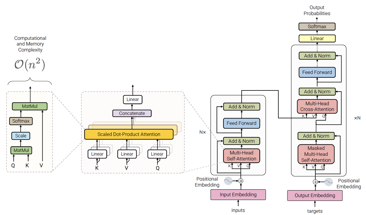
Transformer Extra Parameters
- Input
- = Sequence length
- = Model dimension
- = # of heads
- = /
- Projection matrices , ,
Key, Query, and Value Matrices
Self-Attention and K,Q,V go hand in hand - the intuition for K,Q,V can be seen from an approximate hash table:
- To lookup a value, queries are compared against keys in a table
- In the Hash Table below, there's exactly one K:V pair for any Q
- In contrast for self attention, each Query is measured against all Keys, and the amount of that overlap is assigned to the Values
- Thus attention is a sum of values weighted by K-Q match is returned over the V's
This setup allows us to create a paradigm of:
- Queries (Q):
- Represents the word being attended to / compared to
- Used to calculate attention scores with all Keys
- Key (K):
- Represents all other words (context words) being compared to the Query
- Used to compute the relevance of each context word to the Query
- Value (V):
- Another representation of the context words, but separate and different from Keys
- Although the same input context words are multiplied by 2 different K, V matrices, which results in 2 different Key and Value vectors for same context word
- It basically is a representation of each "word" so at the end, a scored
SUM()of all words is over values! - Weighted by the attention scores to produce the final output
- Another representation of the context words, but separate and different from Keys
These matrices are learned during training and updated via backpropagation
K Q V Complexities
In Bahdanau Attention - each decoder is compared to all encoder states
In Transformer self-attention, we compare all tokens to all tokens simultaneously
Which is now a quadratic term, which is where GPU behavior gets interesting
Tokenization
Tokenization is actually a fairly large part that gets looked over for Transformers - authors and creators of most models have utilized Sub-Word Tokenization to reduce overall vocabulary size and ensure out-of-vocabulary tokens are handled well. Instead of replcaing with [UNK] or something else, splitting up the entire vocabulary into different character chunks allows for reusability between ##ing for dining and banking
Byte Pair Encoding is also utilized as a compression technique which iteratively replaces the most frequent pair of bytes in a sequence with a single, unused byte. Instead of merging together frequent pairs of bbytes, the tokenization algorithms will merge together characters or sub-word character sequences that are frequent. That's how the model learns to pull out ##ing as a sub-word, because it's quite frequent!
Training
This model needs actual training to be done on it to learn these frequency word pairings. The algorithm needs to build merge tables and vocabulary of tokens that ultimately will be updated across epochs to create an optimized set of sub-words to tokenize in the future
Training here isn't really on probabilistic modeling, it's actually a greedy approach based on heuristics and counts in the data, but a new tokenizer would be needed for an inherently unique document set. Doctor shorthand wouldn't be tokenized properly compared to APA structured student essays
The initial vocabulary consists of characters and an empty merge table, at this exact intro step each word is segmented as a sequence of characters, and then the algorithm below is continuously ran:
- Count pairs of symbols - how many times does each pair occur together in the training data
- Find the most frequent pair of symbols
- Merge that pair together in the merge table, and add the new token to the vocabulary
The main parameter to set is the maximum number of merges desired in output merge table, as it ensures you don't over-do merging and lose out on information
The above shows how a vocabulary of cats, mats, mate, ate, etc get turned into merged words separated by the @@ symbols which represent concatenation. In most tokenizers today the separator is ##
Inferece
After learning BPE rules, the merge table is the main artifact output that is reused across inference. The algorithm will segment new words into sequence of characters, and after that iteratively runs over the word running below steps until no other merge is possible:
- Among all possible merges, find highest in merge table
- Run that merge
- Stop if no new merge is able to be found
So inference is just constantly replacing merges over time, and hypothetically could replace an entire word with a compressed single token in some cases
Encoding Blocks
Once we have tokenized inputs relating to some sort of static embedding, we focus on encoding
The main layer you focus on in our Encoding blocks is Self Attention, but alongside this there are other linear layers that help to stabilize our context creation
Self Attention
Self Attention allows words in a single sentence / document to attend to each other to update word embeddings in itself. It's most commonly used when you want a sentence's word embeddings to be updated by other words in the same sentence, but there's nothing stopping us from using it over an entire document.
It was born out of the example of desiring a different embedding outcome of the word bank in:
- The river bank was dirty
- I went to the bank to deposit money
Via Self Attention, the word "bank" in the two sentences above would be different, because the other words in the sentence "attended to" it
Self Attention is a mechanism that uses context words (Keys) to update the embedding of a current word (Query). It allows embeddings to dynamically adjust based on their surrounding context.
Lastly, there are still limitations to Attention, and Attention is not "all you need" at the end of the day!
- It is simply a weighted average, so non-linearities are impossible without further non-linear activation functions inside of neural net
- Bidirectionality may not always be desired (this is covered more in Masked Self Attention)
- Self Attention by itself does not keep word position, and so it's essentially a bag-of-words once again
All of the above are solved via the Transformer Architecture itself outside of Self Attention! This is why transformer encoder and decoder architecture consists of multiple layers of self attention with a feed forward network and positional encodings!
- Residual connections pass "raw" embeddings directly through next layers which helps to prevent forgetting or misrepresenting information
- Layer normalization helps to relieve parameters of given layer shifting because of layers beneath it
- This ultimately reduces uninformative variation and normalizes each layer to mean zero and standard deviation of one
- Scaling down the dot product helps to stop the dot product from taking on extreme, unbounded values because of this variance scaling
Consider the phrase "fluffy blue creature." The embedding for "creature" is updated by attending to "fluffy" and "blue," which contribute the most to its contextual meaning
Self Attentions Complexity is dominated by the sequence length term, and results in because all tokens attend to all other tokens in the sequence
How Self Attention Works
-
The Query vector represents the current word
-
The Key vector is an embedding representing every other word
- Multiply the Query by every Key to find out how "similar", or "attended to" each Query should be by each Key
-
Then you softmax it to find the percentage each Key should have on the Query
-
Finally you multiply that softmaxed representation by the Value vector, which is the input embedding multipled by Value matrix, and ultimately allow each Key context word to attend to our Query by some percentage
-
At the end, you sum together all of the resulting value vectors, and this resulting SUM of weighted value vectors is our attended to output embedding
-
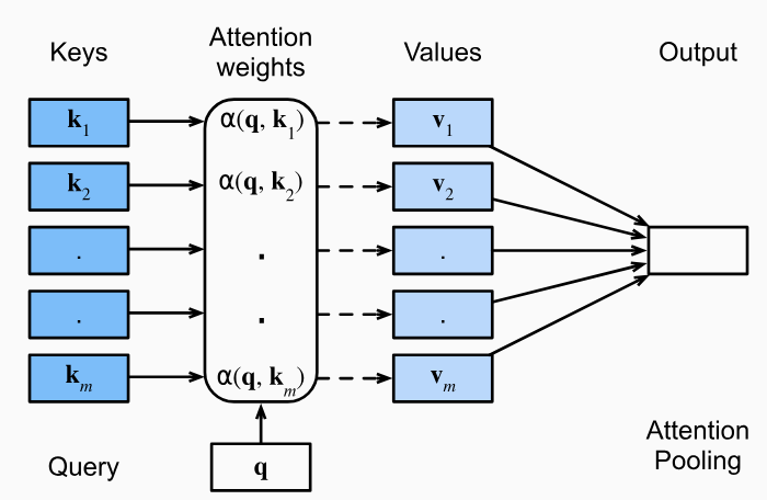
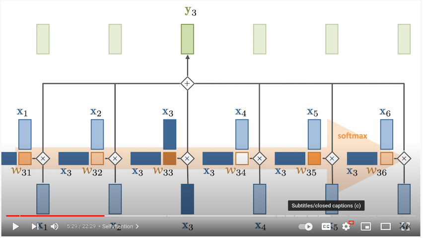
In the below example:
- The dark blue vector from the left is the Query
- The light blue vector on top are the Keys
- you multiple them together + softmax
- Multiply the result of that by each Value vector on the bottom
In depth mathematical explanation below
- Input Transformation:
- Each input embedding is transformed into three vectors: Query (Q), Key (K), and Value (V)
- These are computed by multiplying the input embedding with learned weight matrices:
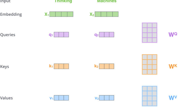
- Self-Attention Calculation:
- Compute attention scores by taking the dot product of the Query vector with all Key vectors :
- Scale the scores to prevent large values:
- Where is the dimensionality of the Key vectors
- As the size of the input embedding grows, so does the average size of the dot product that produces the weights
- Remember dot product is a scalar value
- Grows by a factor of where = num dimensions
- Therefore, you can counteract this by normalizing is via as the denominator
- Apply softmax to convert scores into probabilities:
- Compute the weighted sum of Value vectors:
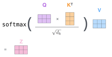
- Output
- The output is a context-aware representation of the token , influenced by its relationship with other words in the sequence
Single Head Self Attention Complexities
RNN's were sequential over , but they only had an compute cost per step. Each decoder hidden state would multiply itself by every encoder hidden state, which was size , roughly relating to . So the path length, referring to the number of sequential steps, was , and at each step there was work done
In self-attention, the path length is reduced to as all of the comparisons are done in parallel, there's nothing sequential! However, at each step (there's only 1 large matrix step) there's work done as we multiply every query by all keys
- RNN:
- Path length
- Compute per step
- Self attention:
- Path length
- Compute per step
Overall, single head time complexity will resolve to
So when
- Sequence length dominates projection size , the quadratic term dominatesd
- When the projection size dominates sequence length , the projection term dominates
Storage is usually the ultimate bottleneck in processing, and the memory complexity of a single head is
Single Head Projection Complexities
Each token
Is multiplied by projection matrices
The total cost per projection, defined as all inputs in sequence of size multiplied by a single matrix of size , is
Since there are 3 matrices total
Single Head Attention Score Complexities
First we need to compare all queries to keys
- So is
- Second one transposed
So the operation has time complexity
After that, we softmax over the matrix
And finally perform weighted value aggregation , which is
Therefore, the entirety of a single-headed self attention time complexity is
Where we assume and
The path length is still because all tokens attend to each other in parallel
Single Head Memory Complexities
The attention matrix itself is an matrix, and so memory ultimately is
This is often the true bottleneck in most transformer architectures when becomes large (this is the large context length problem). Attention is often memory bound at large due to O(S^2)$ attention matrix, even if compute utilization appears high
The bottleneck is:
- Storing attention matrix
- Moving it through HBM
- Reading and writing intermediate tensors
This becomes critical for optimizing later on with things like:
- FlashAttention
- KV Caching
- etc
For example, long-context models begin to show signs of degredation when their GPU utilization is 90% but their FLOPS are stagnant at an unoptimal place like 50%. At this point the GPU is busy working through memory buffers and bringing data into main memory, and it's not able to truly run things in parallel.
Multi-Head Attention
- Instead of using a single set of , Multi-Head Attention uses multiple sets to capture different types of relationships between words (e.g., syntactic vs. semantic).
- Each head computes its own attention output.
- Outputs from all heads are concatenated and passed through a final weight matrix :
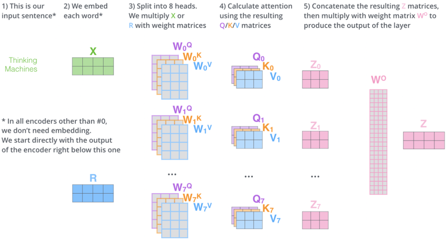
- Outputs from all heads are concatenated and passed through a final weight matrix :
Multi Head Complexity
Single head was
With heads, we now have for each head becuase
Therefore, multi-head attention has the same time complexities as single headed
Pruning
There's an entire section in some Transformer papers talking about pruning of heads. Ultiamtely this is because not every head is needed, and some generally won't have any useful features in some datasets
Pruning allows the model to run faster, perform less computations, and potentially do this without any loss of quality! Most of the time it's a pruning + speed / accuracy tradeoff where you can prune up to certain elbow thresholds where the return on pruning starts to decrease compared to decrease on accuracy
The model needs to be trained with all possible heads being updated, but afterwards pruning is a typical optimization step for production models
Other Layers
Other layers outside of attention based layers in transformers help to extend the problems to a wider set of real world scenario's:
- Non-linearity (feed forward + residual layers)
- Gradient issues (Normalization)
- Distribution shift (normalization, skip layers)
- etc..
Below blurb helps to showcase some of the reasons why all of these layers and architectures are added into the "attention only" architectures (i.e. attention isn't all you need, and below explains why)
One of them is to pass the "raw" embeddings directly to the next layer, which prevents forgetting or misrepresent important information as it is passed through many layers. This process is called residual connections and is also believed to smoothen the loss landscape. Additionally, it is problematic to train the parameters of a given layer when its inputs keep shifting because of layers beneath. Reducing uninformative variation by normalizing within each layer to mean zero and standard deviation to one weakens this effect. Another challenge is caused by the dot product tending to take on extreme values because of the variance scaling with increasing dimensionality . It is solved by Scaled Dot Product Attention, which consists of computing the dot products of the query with its keys, dividing them by the dimension of keys, and applying the softmax function next to receive the weights of the values.
Attention learns where to search for relevant information. Surely, attending to different types of information in a sentence at once delivers even more promising results. To implement this, the idea is to have multiple attention heads per layer. While one attention head might learn to attend to tense information, another might learn to attend to relevant topics. s
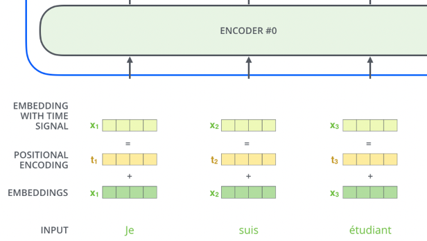
Positional Encoding
- Since Self Attention does not inherently consider word order, Positional Encoding is added to input embeddings to encode word positions
- Positional encodings are vectors added to each input embedding, allowing the model to distinguish between words based on their positions in the sequence
- Why is sinusoidal relevant and useful?
- Allows Transformer to learn relative positions via linear functions (e.g., can be derived from )
- you all know neural nets like linear functions! So it's helpful in ensuring a relationship that's understandable
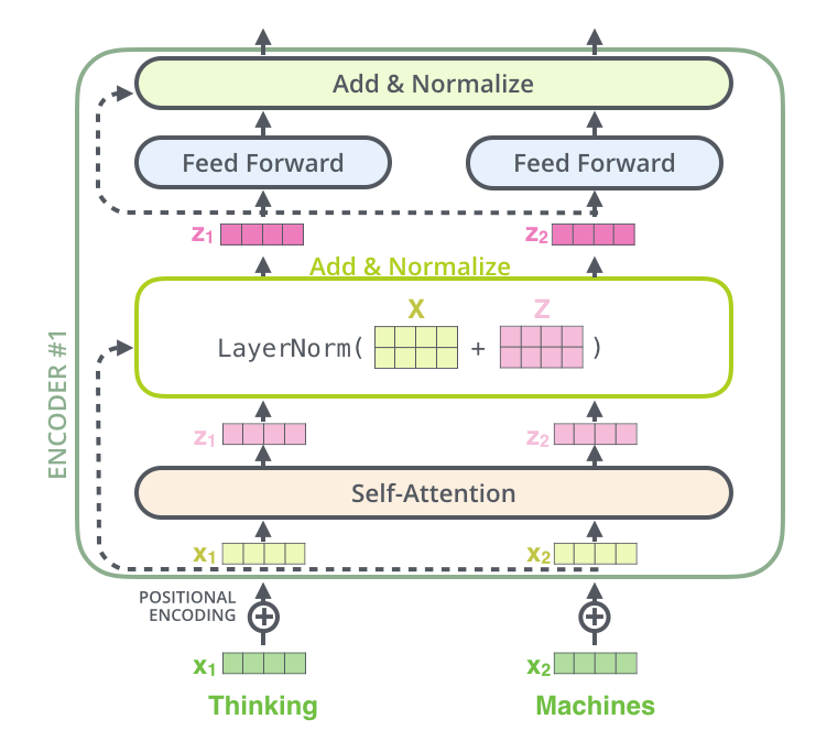
Residual Connections and Normalization
- Each encoder layer includes a residual connection and normalization layers to stabilize training and improve gradient flow
- This happens after both Self Attention Layer and Feed Forward Layer in the "Add and Normalize" bubble
- Add the residual (the original input for that sublayer) to the output of the sublayer
- In the case of Self Attention layer, you add the output of Self Attention to the original input word (non-attended to word)
- Apply LayerNorm to the result
- This just means normalize all actual numeric values over the words embedding
- **If the diagram shows a block over the whole sentence, it just means the operation is applied to all words, but always independently for each word
- Why is any of this useful:
- Helps with gradient vanishing and exploding, and also ensures input stability
Summary of Self Attention Encoding
-
Input Embedings:
- you take our input words, process them, and retrieve static embeddings
- This only happens in the first encoding layer
-
Positional Encoding:
- Add positional information to embeddings to account for word order
-
Self Attention: 3.1 Input Transformation:
- Positionally encoded embeddings are transformed into using learned weight matrices.
3.2 Self Attention Calculation:
- Compute attention scores using dot products of and , scale them, and apply softmax.
3.3 Weighted Sum:
- Use the attention weights to compute a weighted sum of , and add that onto the input word, producing the output.
3.4 Residual + Normalization:
- LayerNorm add together input and self-attended to matrices
3.5 Feed Forward Layer:
- Each position’s output from the self-attention layer is passed through a fully connected feed-forward neural network (the same network is applied independently to each position)
- Essentially just gives model another chance to find and model more transformations / features, while also potentially allowing different dimensionalities to be stacked together
- If you have 10 words in our input, you want to ensure the final output is the same dimensionality as the input
- I don't know if this is exactly necessary
4 Multi-Head Attention:
- Use multiple sets of to capture diverse relationships, then concatenate the results.
This diagram below shows one single encoding block using Self Attention
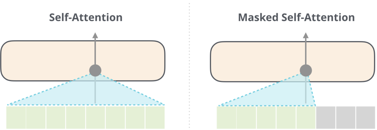
Masked Self Attention
- In Masked Self Attention, it's the same process as Self Attention except you mask a certain number of words so that the results in 0 effectively removing it from attention scoring
- In BERT training you mask a number of words inside of the sentence
- In GPT2 training you mask all future words (right hand of sentence from any word)
Context Size and Scaling Challenges
- The size of the matrix grows quadratically with the context size (), making it computationally expensive for long sequences.
- To address this, masking is used to prevent future words from influencing current words during training (e.g., in autoregressive tasks).
- Context size
- Size of Q * K matrix at the end is the square of the context size, since you need to use all of the Q * K vectors, and…it’s a matrix! So it’s n*n = n^2 so it’s very hard to scale
- It does help that you mask ½ the examples because you don’t want future words to alter our current word and have it cheat
- Since for an entire sentence during training for each word you try to predict the next, so if there are 5 words there’s 1, 2, 3, 4, 5 training examples and not just 1
- Don’t want 4 and 5 to interfere with training 1, 2, 3
Encoder-Decoder Attention
Encoder-Decoder Attention is a mechanism used in Seq2Seq tasks (e.g., translation, summarization) to transform an input sequence into an output sequence. It combines Self Attention within the encoder and decoder blocks each, and then cross-attention between the encoder and decoder
Encoder
Encoder:
- The Encoder Portion is completely described in Summary of Self Attention Encoding
- TLDR;
- The encoder processes the input sequence and generates a sequence of hidden states that represent the context of the input
- Each encoder block consists of:
- Input Embedding:
- The first encoding layer typically uses positional encoding + static embeddings from Word2Vec or GLoVE
- Self Attention Layer:
- Allows each token in the input sequence to attend to other tokens in the sequence
- This captures relationships between tokens in the input
- Feed Forward Layer:
- Applies a fully connected feed-forward network to each token independently
- Typically two linear transformations with a ReLU/GeLU in between:
FFN(x) = max(0, xW₁ + b₁)W₂ + b₂
- Residual Connection + LayerNorm
- Add input / output of layer, and then normalize across vector
- Input Embedding:
- The output of each encoder block is passed to the next encoder block as input, and the final encoder block produces the contextual embeddings for the entire input sequence
- These are further transformed into K, V contextual output embeddings
- This confused me at first, but basically the output of an encoder block is same dimensionality as word embedding input, so it can flow through
- This is usually known as
d_model
- This allows us to stack encoder blocks arbitrarily
- Architecture:
- Composed of multiple identical blocks (e.g., 6 blocks by default, but this is a hyperparameter)
- Each block contains:
- Self Attention Layer: Captures relationships within the input sequence
- Feed Forward Layer: Processes each token independently
Encoder Complexity
Encoder complexities here are the same as self attention complexity
It's based on the sequence length, and projection dimensions
Decoder
Parameters:
- = encoder length
- = decoder length
- = model dimension
- = # of heads
So inside of the masked self attention layer:
Inside cross-attention layer:
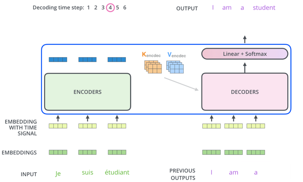
The decoder generates the output sequence one token at a time, using both the encoder's output and its own previous outputs. Each encoder, and specifically the last one, outputs a hidden state matrix that's the size of the sequence and the projected attended to embeddings (i.e. for each input in , we have a vector of size ). Afterwards, each decoder block will apply masked self-attention over the encoder input and the previous decoder outputs, which allows it to auto-regressively focus on it's past output words to predict the next word
- Input:
- The contextual embeddings output from the final Encoding Layer
- These K, V contextual output embeddings are passed to each Decoder block
- For cross-attention, the decoder applies it's own learned to that encoder output
- Keys and Values are re-projected in each decoder layer
- The previous Decoder block(s) output (previously generated word)
- The contextual embeddings output from the final Encoding Layer
- Each decoder block consists of:
- Masked Self Attention Layer:
- Allows each token in the output sequence to attend to previously generated tokens in the sequence (auto-regressive behavior)
- Future tokens are masked to prevent the model from "cheating" by looking ahead
- So self-attention only happens from words on the left, not all Keys
- Query: Current token's embedding
- For the first layer this is the embedding from our actual input
- For deeper decoder layers, this is from the decoders previous output
- Key and Values: All already generated words to the left
- Similar to self-attention except you ignore all to the right
- Encoder-Decoder Attention Layer:
- Attends to the encoder's output (contextual embeddings) to incorporate information from the input sequence
- Query: Comes from the decoder's self-attention output
- i.e. it's the decoder's current representation of a token after masked self-attention
- Key and Values: Encoder's output for each input token
- Feed Forward Layer:
- Applies a fully connected feed-forward network to each token independently
- Masked Self Attention Layer:
- Architecture:
- Composed of multiple identical blocks (e.g., 6 blocks by default).
- Each block contains:
- Self Attention Layer: Captures relationships within the output sequence
- Encoder-Decoder Attention Layer: Incorporates information from the encoder's output
- Feed Forward Layer: Processes each token independently
- Example:
- Input sentence has 5 words in total
- Remember, the encoder put out 5 total vectors, one for each input word
- Let's walk through the third word in the decoder output, meaning the first two have already been generated
- Decoder Self Attention
- Input: The embeddings for the first, second, and third generated tokens so far
- The query is the input embedding (same one fed to encoder) for the 3rd word
- K,V are the input embedding (same one fed to encoder) for the 1st and 2nd words so far
- Masking: The self-attention is masked so the third position can only "see" the first, second, and third tokens (not future tokens)
- What happens: The third token attends to itself and all previous tokens (but not future ones), using their embeddings as keys and values
- Input: The embeddings for the first, second, and third generated tokens so far
- Encoder Decoder Cross Attention
- Input: The output of the decoder’s self-attention for the third token (now a context-aware vector), and the encoder’s output for all input tokens
- Q, K, V:
- The query is the third word's attended to vector (after self-attention and residual/LayerNorm in decoder)
- The keys and values are the encoder’s output vectors for each input token (these are fixed for the whole output sequence)
- What happens The third token’s representation attends to all positions in the input sequence, using the encoder’s outputs as keys and values
- Input sentence has 5 words in total
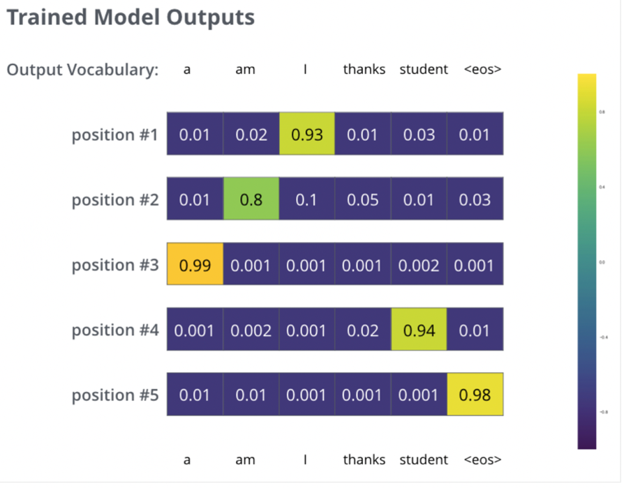
- Final Decoder Output:
- The final decoder layer produces a vector of floats for each token, which is passed through:
- A linear layer to expand the vector to the vocabulary size
- A softmax layer to produce a probability distribution over the vocabulary for the next token
- The final decoder layer produces a vector of floats for each token, which is passed through:
Decoder Complexity
The decoder is more complicated than the encoder!
is the current decoders output so far, and so at each decoder step we utilize these previous outputs and relate them to the input sequence , and the current output
Decoder Training
The decoder has 2 attention blocks:
- Masked self-attention
- Cross-attention
So the total per decoder layer comes to
In this section the sequence length is roughly equivalent to the decoder sentence length. So in total, the time complexity per decoder step is dominated by the sequence size
Decoder Inference
For long-context LLM inference, will grow auto-regressively while it has to continue keeping the full sequence in memory
Masked Self-Attention will reduce to per token if utilizing KV Caching, which is a GPU inference optimization method
Cross attention per token then becomes
So the total per generated token is
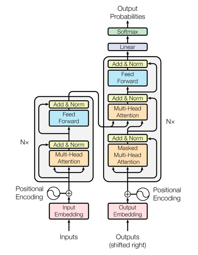
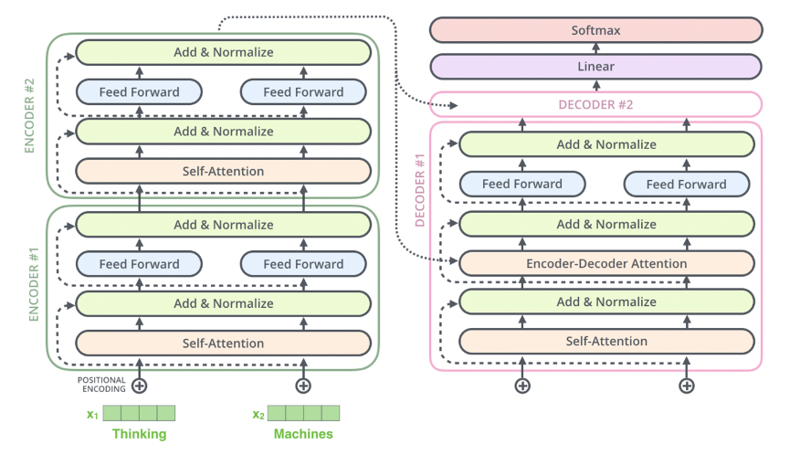
Visual Representation
-
Encoder Block:
- Self Attention → Feed Forward → Output to next encoder block.
-
Decoder Block:
- Self Attention → Encoder-Decoder Attention → Feed Forward → Output to next decoder block.
-
Final Decoder Output:
- The final decoder output is passed through a linear layer and softmax to produce the next token.
- The final decoder output is passed through a linear layer and softmax to produce the next token.
Summary of Encoder-Decoder Attention
-
Encoder:
- Processes the input sequence and generates contextual embeddings using self-attention.
-
Decoder:
- Generates the output sequence token by token using:
- Self Attention: Captures relationships within the output sequence.
- Encoder-Decoder Attention: Incorporates information from the input sequence.
- Auto-Regressive Decoder: Tokens are predicted auto-regressively, meaning words can only condition on leftward context while generating
- Generates the output sequence token by token using:
-
Final Output:
- The decoder's output is passed through a linear layer and softmax to produce the next token.
-
Training:
- The model is trained using cross-entropy loss and KL divergence, with each token in the output sequence contributing to the loss.
- The model is trained using cross-entropy loss and KL divergence, with each token in the output sequence contributing to the loss.
Transformer Optimizations
There's a number of optimizations in this architecture that a lot of production systems use to speed up inference, saturate GPU utilization, and reduce overall size and runtime of the models after training has been completed
- Pruning was already covered where you remove some of the heads in multi-head attention, and this can be done after training with an evaluation set to see if a majority of variance is covered in distinct heads (removing heads 1 and 4 in a set of 12)
- KV Caching is an inference only optimization that caches the results from multiplication during the auto-regressive phase in decoding inference, ultimately allowing to skip all historic calculations for already output words for all future words
- Quantization reduces the overall precision of the data types from
float32to lesser numbers likefloat16orfloat8. The rationale is that during training the extra precision helps with gradient stability, accuracy, and convergence - especially since we are multiplying thousands of numbers in such small ranges (potentially all between[0.00, 1.00]) the extra precision helps to ensure there's no loss of information. Once training is done, and the numbers have converged to allow for latent features, some architectures are able to reduce these data points total size and keep a majority of features and variance preserved- Mixed Precision Training is another "flavor" of this where you use lower precision for most computations while keeping critical parameters as higher precision
- Gradient Clipping caps the gradient to prevent exploding gradients during training - most transformers try and tackle this with residual layer, normalization layer, identity layers, dropouts, etc and gradient clipping is another common tool if gradients start to explode
- Sparse Attention reduces the quadratic complexity of self-attention by attending to only a subset of tokens
- Go from comparisons to where is the length of the subset of tokens we are performing self-attention on
- Architectures will use local tokens, stored global tokens, random sampling, sliding windows, and skip-token self-attention layers to reduce memory and hopefully preserve context needed for self-attention variance
- Flash Attention implements memory-efficient attention by computing attention in chunks to reduce memory overhead instead of putting the entire matrix into memory. Should ultimately help GPU utilization and reduce memory bottlenecks for sequences because the context doesn't grow with generation
- Similar to Sparse Attention where you focus on a local context of tokens
KV Caching
KV Caching comes up in a lot of areas, and interviews, especially around "The GPU is at 90% utilization, but it's FLOPS utilization is stagnant around 30%, what is the first potential cause of this?" where you should dive into memory overheads on GPU's and try and see if there's redundant memory bottlnecks on a GPU that's causing too much shuffle and not allowing SIMD operations to run. One way to alleviate this issue is with KV Caching, where you reuse a number of the operations computed in the auto-regressive decoder inference portion of LLM modeling
As a sentence moves forward, the input is [prompt], and over time more and more output words are computed - [prompt] + y_1, [prompt] + y_1 + y_2, ... so on. Each of the new output tokens y_1, y_2 will continuously be involved in both cross-attention and self-attention operations, and so during this phase we can cache these results over each inference period in GPU cache and reuse them until we are complete with a round of inference
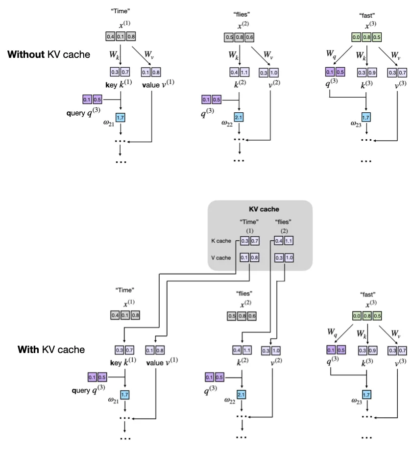
This will utilize GPU Buffers, which are essentially dedicated blocks of memory used for storing WORM based vectors - sometimes they are write-once, other times they can be overwritten, but typically in caching you don't want to be continuously writing to them. If they aren't present, simply store them on the fly and continue
Show Python Script
def forward(self, x, use_cache=False):
b, num_tokens, d_in = x.shape
keys_new = self.W_key(x) # Shape: (b, num_tokens, d_out)
values_new = self.W_value(x)
queries = self.W_query(x)
#...
if use_cache:
if self.cache_k is None:
self.cache_k, self.cache_v = keys_new, values_new
else:
self.cache_k = torch.cat([self.cache_k, keys_new], dim=1)
self.cache_v = torch.cat([self.cache_v, values_new], dim=1)
keys, values = self.cache_k, self.cache_v
else:
keys, values = keys_new, values_new
Sparse Attention
TODO:
Flash Attention
TODO:
Vision Transformers (ViT)
In using transformers for vision, the overall architecture is largely the same - flattening structure out and using augmention for new examples and then doing self-supervised "fill in the blank" for training
All changes are relatively minor:
- Input:
- Text: Input is a sequence of tokens
- Vision: Input is an image split into fixed size patches
16x16- Each patch gets flattened and linearly projected to form a "patch embedding" similar to static word embeddings
[CLS]token used for classification tasks
- Positional Encoding:
- Text: Added to token embeddings to encode word order
- Vision: Added to patch embeddings to encode spatial information of each patch in the image
- Objective:
- Text: Predict the next word (causal), fill in the blank, or generate a sequence (translation / summarization)
- Vision: Usually image classification, or can also be segmentation, detection, or masked patch prediction (fill in the blank)
- Architecture: Basically the same without any major overhauls
- Self Supervision:
- Text: Fill in the blank, next sentence prediction
- Vision: Fill in the blank (patch), or pixel reconstruction which aims to recreate the original image from corrupted or downsampled versions