Embeddings

Embeddings

Embeddings are dense vector representations of objects - typically you use them for Documents, Queries, Users, Context, or Items...but they can really be used to represent anything

History

• In the past there have been many ways of creating embeddings
• Encoders
  • One Hot Encoding: When you would replace categorical variables with vectors of sparse 0's and a single 1 representing the category
  • Binary Encoders: Converts categorical variables into binary code - similar to One Hot Encoding, except you basically pick an ID that incrementally increases for new categories
• Collaborative Filtering is discussed later on
• Word2Vec
• Doc2Vec
• Node2Vec!
• etc...

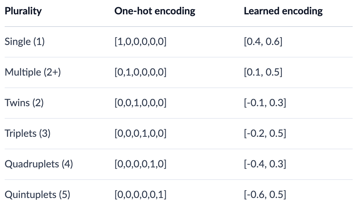
Categorical Embeddings

ML models typically need fixed length vectors as their input, and over time they look to create distributions over these input

With a dictionary of words it's hard to think about the best way to set up these fixed length vectors, and the first attempt was One Hot Encoding where you'd simply have a sparse vector with 1's all around where your words were

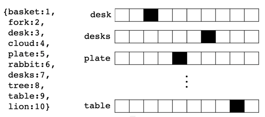
• One-Hot Encoding represents orthonormal basis of vectors, and typically is useful for categorical variables but becomes infeasible if you try to use it for text features
• Label Encoding is similar to One-Hot Encoding, except you use an incremental ID for each of the categories

Pitfalls

Common pitfalls associated with these categorical embeddings is that:

• They create humongous vector spaces of orthogonally independent vectors
  • Essentially each vector is a different basis vector at this point
  • This eventually results in the common curse of dimensionality issue where data becomes too sparse and models stop learning / updating
• Having these sparse, orthogonal vectors means you cannot generalize easily
  • There's no good way to generally compare words for similarities, as you cannot comapare [1,0] to [0,1] in a general fashion over millions of vectors

Therefore, these sorts of categorical embeddings can be made better by use of dense embeddings over a smaller overall dimensional space (i.e. less dimensions, with more information "squished" into each dimension)

From this, word embeddings ultimately moved towards dense representations of floating point numbers, known as Text Embeddings where the dimensionality of embeddings is typically much smaller than the number of words in the dictionary which allows for space reduction, information gain, and geometric comparisons

Numeric Features

• Standardization: Transforms the data to having a mean of zero, and a standard deviation of one
  • This allows us to bring data in different distributions onto the same common scale
  • $[ z = \frac{x - \mu}{\sigma} ]$
• Normalization: Brings the data to a specific range between $[0, 1]$
  • This is helpful when you want to ensure all features contribute equally to the model
• When to use what?
  • Standardization:
    • Use when the features have different units or scales
    • Useful for algorithms that assume the data is normally distributed (e.g., linear regression, logistic regression, SVM)
    • Helps in dealing with outliers.
  • Normalization:
    • Use when you want to scale the data to a specific range (e.g., [0, 1])
    • Useful for algorithms that do not assume any specific distribution of the data (e.g., k-nearest neighbors, neural networks)
    • Ensures that all features contribute equally to the model
• There are plenty of other ways to treat numeric data as features, but not covering them here

Text Embeddings

Text Embeddings are one of the harder things to figure out, but there are some standards nowadays

Text embeddings can be seen as a static form of transfer learning, where models will create static word embeddings and over time anyone can re-use these via a lookup object for any word - the word "bank" in terms of river bank, or financial institution, will have the same embedding here

• Training Word2Vec and BERT both involved semi self-supervised training where they take online corpus as input and basically use contextual words $w_{i-k,i+k}$ to try and create an embedding for a current word $w_i$
• Word2Vec was one of the original ideas for text embeddings - it essentially acts as an autoencoder to create static embeddings for each word in a dictionary
• BERT on the other hand, through attention, can create contextual embeddings for words, sentences, and entire documents
• GPT is an autoregressive transformer model in the same transformer "family" as BERT, but it is unidirectional where BERT is bidirectional (which is constantly repeated in the paper)
  • GPT is good for text-to-text tasks like question answering, but like BERT you can pull from the middle hidden layers during it's self-attention steps to find word embeddings

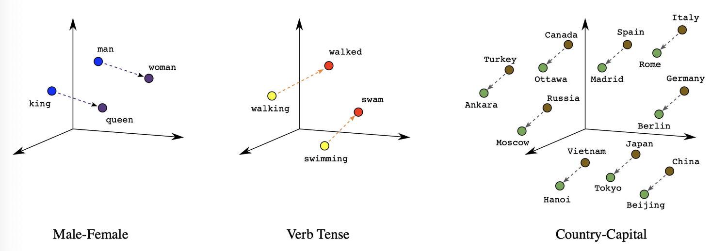
Word Embeddings made it possible and allowed developers to encode words as dense vectors that capture underlying semantic content - King - Man + Woman = Queen. Similar words were embedded close to each other in lower dimensional feature spaces, and allowed for geometrical operations.

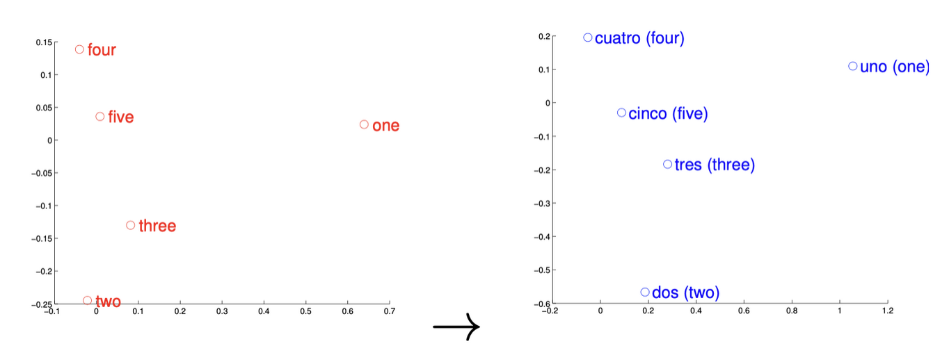
These examples have even been shown to hold across languages, where youc can map One $\rarr$ Uno - this ultimately showed 90% precision across words, and showcases that some languages may have an isomoprhic (one-to-one and onto) topological mapping for some % of their words. Other languages like English $\rarr$ Vietnamese has a much lower overlap, showcasing a relatively small one-to-one correspondence because the concept of a word and meanings of them are vastly different in the 2 languages. I still think this is one of the more interesting case studies; Other groups took this further and removed words from the vocabulary and retrained the models and were able to find "missing vectors" of the vocabulary words they had taken out that were "missing" in the one-to-one translation

Word2Vec

Word2Vec is a family of algorithms and techniques to create static embeddings

It will create dense embeddings for all words, subwords, or tokens in vocabulary, and then they can be used in the future for many downstream tasks - if you have static embeddings for all words in a sentence, you can average / add / min-max or something else to create a sentence embedding. These embeddings are static though, so the embedding for bank is the same regardless of if it refers to a river bank or a financial institution

• Parameters:
  • $N$ is context window size (input size)
  • $V$ is the number of words in our dictionary
  • $D$ is the embedding size (projection layer)
  • $i$ is the current target word

Training and Output

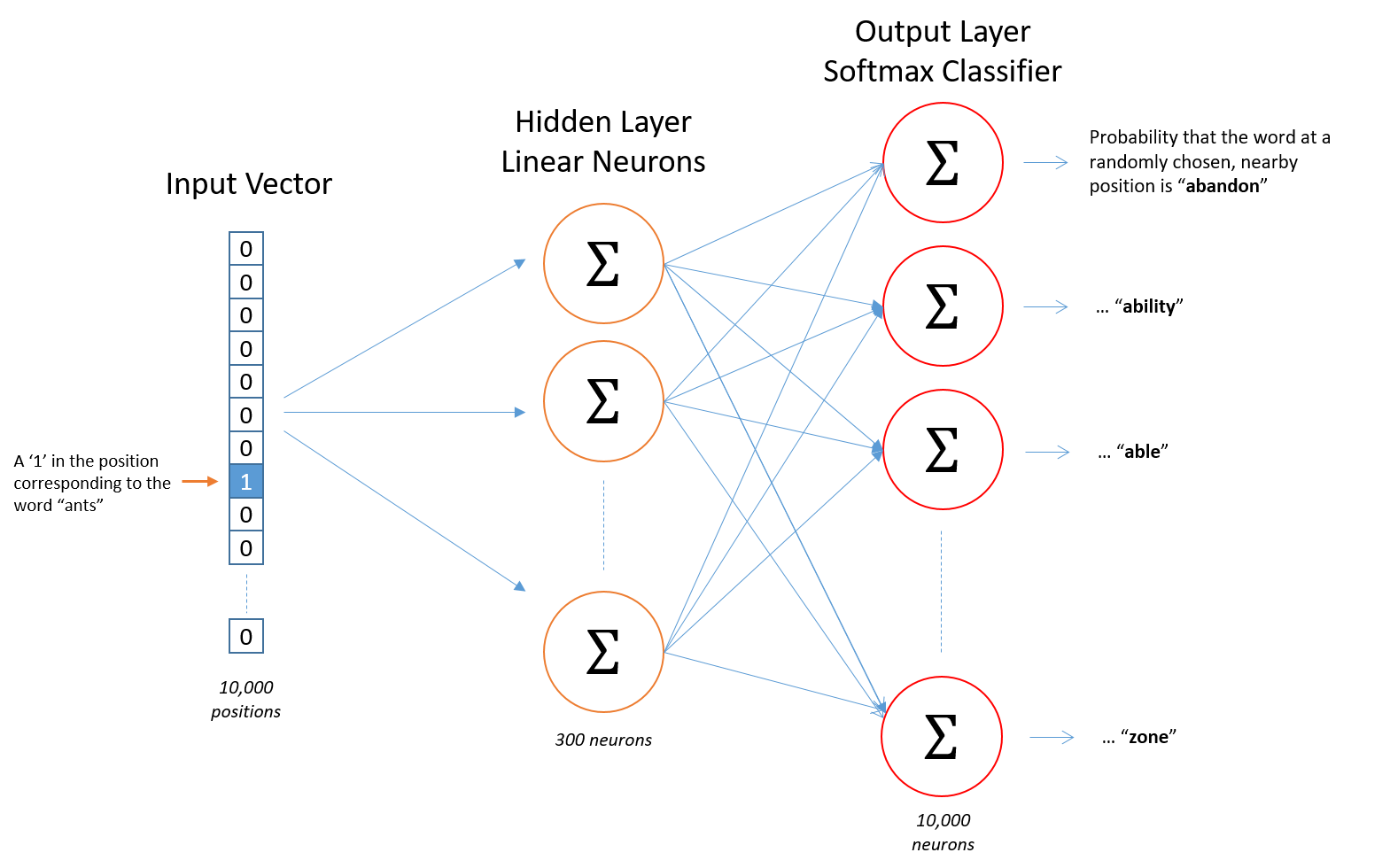
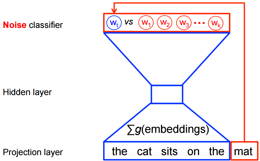
Word2Vec is shallow 2 layer NN trained on a vocabulary of texts and tokens. Typically words are tokenized out into sub-words which ultimately reduces the total size of the corpus. #ing is a common token, which can be paired with cook, read, fish, etc instead of duplicating all of those words in different contexts

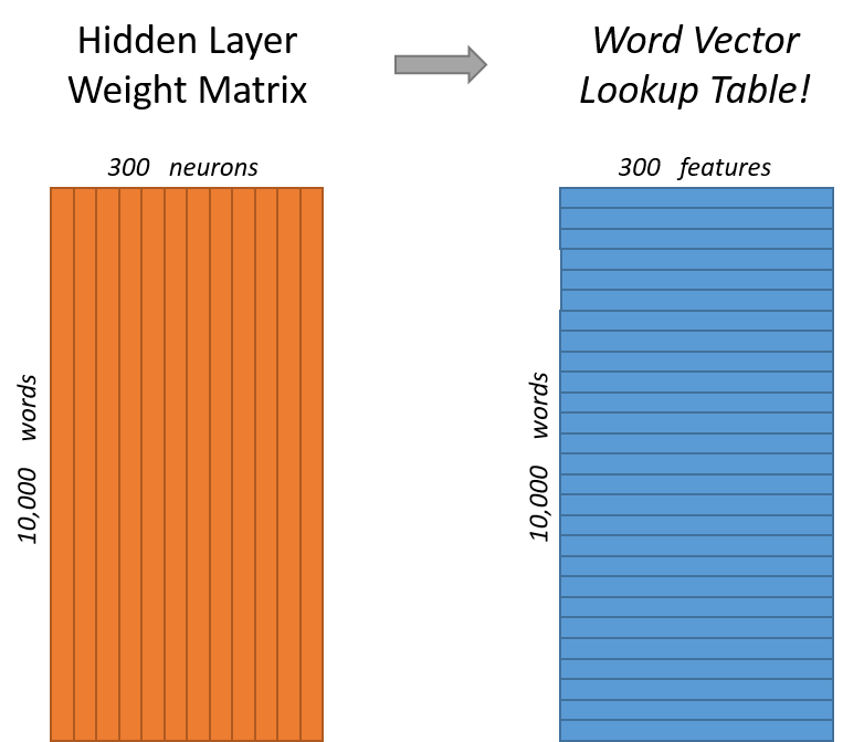
The training architecture is meant to update middle hidden layers of word representations by altering them in geometric space so that downstream objectives lower their loss, and in doing this eventually the middle hidden layers will actually just become the token embeddings themselves, and we can trash the later layers. These hidden layers are updated by multiple objectives like CBOW, Skip-Gram, and other methods in the Word2Vec family, and the sampling, objectives, and architecture tweaks help to optimize the total runtime of the model and prevent overfitting

Training hidden layers with different objectives, and then utilizing those hidden layers as embeddings, is a common practice in semi-supervised learning. There is no exact output for each input word, but you can create actuals via context and surrounding words. Many other areas of self semi-supervised learning are grouped into this - autoencoders will try and reduce dimensionality and compress objects by producing an encoding hidden layer, and contrastive learning is an objective where you augment inputs and try and predict the original and augmented pairing - you can use transformations, context, etc to generate pairs to update model weights on, without having explicit labeled training data

Model Architecture and Optimizations

Word2Vec has a similar architecture to an autoencoder where you take a large input vector, compress it down to a smaller dense vector, and then instead of decompressing it back to the original input vector (which is what's done with autoencoders), W2V outputs probabilities of target words

Inputs to W2V are one-hot encoded vectors, because you have to start somewhere with some sort of input. The hidden layer is a standard fully-connected (dense) layer, and the output layer consists of probabilities for target words from the vocabulary

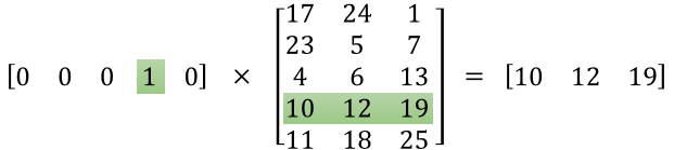
For the CBOW architecture, we take $N$ input context words and produce a singular output representing our predicted current word:

• Input Layer:
  • One-hot encoded vectors representing the word
  • If our vocabulary is size $V$, the dimension of the input would also be $V$, and the input is a sparse vector of all 0's and a single 1
  • $N \times V$
    • $N$ examples will come in via context words
    • For each of these $N$ context words, we will need a one-hot encoded vector of size $V$
• Hidden Embedding Layer:
  • $V \times D$
    • Will need to transform the $N \times V$ layer via fully connected dense transformations into our lower dimensional embedding layer
  • The output will be $N \ times D$ where we have a weighted row for each of the $N$ inputs
  • 
• Output Layer:
  • General purpose usually consists of softmax classifiers
  • $N \times D$ input from hidden layer will be output to $V \times 1$
  • Basically, the output is a single vector of size $V$ with probabilities assigned to each word

For each input word we'll multiply it by the current representation embedding, so in the below ants and cars example the input $\rarr$ hidden embedding multiplication can be interpreted as "how similar is ants vector to cars vector"

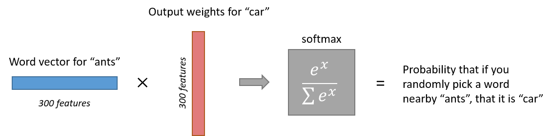
If ants and cars are similar, then this resulting output will be larger and will influence softmax to choose cars instead of another word. Most likely ants will be closest with a word like insect or bug, and softmax loss function will update the weights to become closer to those representations over each backwards update to weights

Optimizations

To run the actual above technique is computationally expensive, as you'd need to compute and normalize all vocabulary words at each training step which isn't necessary. Negative sampling and hierarchical softmax allow us to update words and compute outputs for only a small set of context words and "other words" which makes this much more feasible at a larger scale - you don't need to update the embedding for "Mexico" for the input word "chair" (most likely), and so negative sampling, hierarchical softmax, etc all revolve around those optimizations

• Hierarchical Softmax uses a Huffman Tree to reduce overall calculation by approximating the conditional log-likelihood at the ending softmax classification layer
  • Huffman tree's help us to get to utilizing $log_2(V)$ memory complexity instead of full $V^2$ that would be needed for comparing every vocabulary word to every other one
  • As training epochs increase, hierarchical softmax stops being useful
  • TODO write more in softmax area on loss and link here
• Negative Sampling samples $\hat{N}$ negative instances along with the actual target word $y$ inside of the total context $N$. Negative sampling helps to ignore most of the "0" in the one-hot encoded vectors and resulting vocabulary, and so we only have to propogate weight updates to $\hat{N}$ instances instead of the entire $V$ vocabulary during each backwards pass
  • Negative sampling samples negative instances (words / tokens) along with the target word and minimizes the log-likelihood of the sampled negative instances while maximizing the log-likelihood of the target word
  • Negative samples are typically chosen using a unigram distribution, which intuitively means the probability for selecting a word as a negative sample is related to it's frequency. More frequent words are more likely to be sampled as negatives
    • Each word is given a weight equal to it's frequency (word count) raised to the #3 \over 4$ power, and then the probability of any word is it's weight divided by the sum of weights for all words
  • 
• Sub Sampling is a technique to avoid calculating extremely frequent words / tokens such as it, is, a, the, etc..
  • These more frequent words won't provide much more information, and so ideally they are skipped over more often during training to speed up the process
  • Words above a certain threshold can be sub-sampled to increase training speed and performance
• Curse of Dimensionality comes up as larger dimensional vectors will produce better embeddings up to a certain threshold, where afterwards the quality starts to rapidly diminish in terms of quality increase per dimension increase
  • Typically the dimensions are set between 100 and 1,000

The hidden layer is size $V \times D$, because we'll need to represent all $V$ words with some potential weight matrix

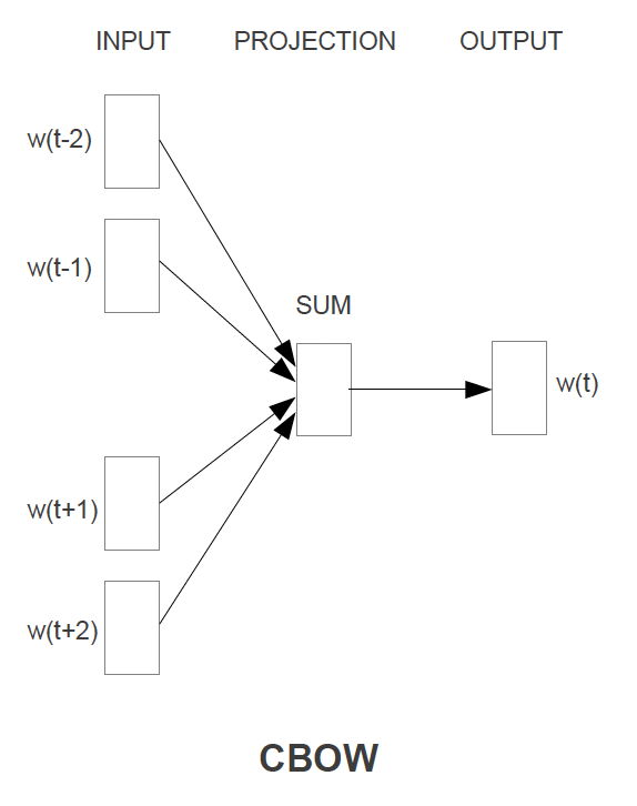
Continuous Bag of Words Architecture

The CBOW architecture will use some surrounding context of words, $w_{i-N//2,i+N//2}$, to predict the current word $w_i$

• The context words get projected into hidden layer, and then they are basically all averaged
  • This means there is no context involved, and that the surrounding words are simply averaged
• For the $N$ context words, past and future words are used
  • In the paper $N == 8$ with 4 before (historic), and 4 after (future)
• Training Objective: Predict the middle word from the $N$ surrounding context words
• Time Complexity: Would be $TC = N \times D + D \times log_2(V)$
  • General rule of thumb: Pluses separate layers, multiplication shows layer dimensions / work
• The output layer is a log-linear classifier
  • TODO: Explain log-linear classification
• 

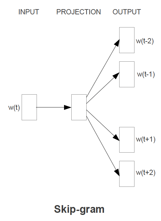
Continuous Skip Gram Architecture

The Skip Gram architecture will use the current word $w_i$ as input to predict each one of the context words $w_{i-N//2,i+N//2}$

• The current word is sent through a log-linear classifier into a continuous projection layer, and then they projection layer is used to predict the best potential context words
  • This still! means there is no context involved, and that the surrounding words are simply predicted without specifying placement
• Training Objective: Predict some $C : C \leq N$ surrounding context words from the current word, and then pick, randomly, $C$ words from the $N$ context words
  • Since more distant words are most likely more unrelated to the current word, you reduce computational complexity by sampling from those words less frequently
  • There's no other way to give less weight to other "far away" words other than sampling them less and updating weights less often based on them
• Time Complexity: Would be $TC = C \times D + C \times D \times log_2(V) === C \times (D + D \times log_2(V))$
  • For each of the $C$ words you need to take our input word $w_i$, do $D$ multiplcations to get it into projection layer, and then go from our projection layer into our sized $V$ vocabulary to try and predict $w_c$
• 

Evaluation of Model

Evaluating an embedding model is a subjective process over each evaluation objective - do you want to check words having a 1:1 mapping over languages, or check for semantic similarity, or even something else like word clustering. Each objective function needs to have evaluation datasets, and

• In the past the main way to do this was to just show tables of words with their corresponding Top-K most similar other words, and intuitively check

• In the Word2Vec Paper they checked over relationships such as "What is the word that is similar to small in the same sense as bigger is to big"

  • Ideally this would produce smaller

• This can be done with algebraic operations! vector(big) - vector(bigger) + vector(small) would give us that sort of output, and then you just find the closest vector via Cosine Distance

• There are other relationships to test such as France is to Paris as Germany is to Berlin

• Skip Gram performed better on semantic objectives, which isn't surprising seeing as it's entirely focused on structuring a word to best represent what other words would be around it, so America and United States should be similar

  • Skip-gram also typically performs better on larger datasets, and continuously has the highest accuracy metrics on most datasets

• Bag of Words performed better on syntactic objectives showing how the CBOW model is better at syntax modeling where you could alter the sentence The quick brown fox jumped over the lazy river to Over the lazy river the quick brown fox had jumped

  • CBOW produces similar, but worse, accuracy metrics compared to skip-gram, but is much more computationally efficient

Encoder Decoder

Over time word embeddings and sentence embeddings were gaining traction, but things became awkward when there wasn't a fixed length 1:1 mapping from input to output. "My name is Luke" $\rarr$ "Me llamo Luke" isn't a 1:1 mapping, and so machine translation and other similar tasks started hitting these sequence-to-sequence roadblocks

Ultimately, the thought process was to build an architecture with 2 parts:

• Encoders dealt with variable length input sequences to transform it into a fixed state / fixed size vector
• Decoders would take that fixed size hidden state, and output a variable length output

These could utilize Recurrent NN's for variable length input and output, or really any other architecture that allowed for repeating predictions, and then the mapping between variable length sequence to variable length sequence could be achieved

The generic framework proposed in initial papers has:

• Encoder RNN processes the input sequence of length $n_{x}$ to compute a fixed length context vector $C$
  • This context vector is usually just the final hidden state of the encoder, or some function of the hidden states if that's desired
  • This context vector is supposed to encode all relevant information, signals, etc about the input vector
• Decoder RNN process uses the context vector to produce a target sequence of length $n_{y}$
  • The context is passed to every hidden state of the decoder, the decoder RNN uses this information to produce the target sequence of length $n_{y}$, which can of course vary from $n_{x}$

Encoder

The encoder portion is really just a straightforward RNN! It's main objective is to output a hidden state context vector $c$, and to be able to handle varying length inputs and preserve their signal in $c$

Each input (let's say one single sentence) will have multiple words / tokens, where each token is represented by a fixed size embedding (most likely something from Word2Vec) - each input feature vector $\bold{x}_{t}$ can be represented as a static word embedding for the rest of this article

At any time step $t$, the RNN transforms the input feature vector $\bold{x}_{t}$ for token $x_t$, and also uses the hidden state $\bold{h}_{t - 1}$ to create the current hidden state $\bold{h}_{t}$

$$\bold{h}_{t} = f(\bold{x}_{t}, \bold{h}_{t-1})$$

This will happen over each of the input tokens, and ultimately we will use the set of hidden states $\{\bold{h}_{0}, \bold{h}_{1}, ..., \bold{h}_{T}\}$ to create the final hidden state $c$

$$c = q(\{\bold{h}_{0}, \bold{h}_{1}, ..., \bold{h}_{T}\})$$

$q$ can be an identity function, which means $c$ is just the final hidden state, or it can aggregate all of the hidden states, use some weighted aggregation, etc

The example above utilizes a unidirectional RNN, but the same encoding process can be done with a bi-directional encoder as well. As long as it makes sense in the context of the overall architecture, we might as well utilize the extra information! In that case we would simply do the unidirectional pass in both directions, and then any hidden state would be a function of it's 2 unidirectional passes

$$\bold{h}_{t} = f(\overrightarrow{\bold{h}_{t}}, \overleftarrow{\bold{h}_{t-1}})$$

Below python snippet showcases how you can use an Embedding layer (word2vec or modern equivalent) along with some generic rnn calls to create a forward pass of an encoding layer

Show Python Script

class Seq2SeqEncoder(d2l.Encoder):  #@save
    """The RNN encoder for sequence-to-sequence learning."""
    def __init__(self, vocab_size, embed_size, num_hiddens, num_layers,
                 dropout=0):
        super().__init__()
        self.embedding = nn.Embedding(vocab_size, embed_size)
        self.rnn = d2l.GRU(embed_size, num_hiddens, num_layers, dropout)
        self.apply(init_seq2seq)

    def forward(self, X, *args):
        # X shape: (batch_size, num_steps)
        embs = self.embedding(X.t().type(torch.int64))
        # embs shape: (num_steps, batch_size, embed_size)
        outputs, state = self.rnn(embs)
        # outputs shape: (num_steps, batch_size, num_hiddens)
        # state shape: (num_layers, batch_size, num_hiddens)
        return outputs, state

Decoder

The decoder is a much more interesting part to focus on, as it starts to incorporate many new architectures that will eventually underpin things like Self Attention and contextual embeddings

At each time step $t'$ the decoder assigns a probability to each possible token in the vocabulary, and the probability is conditioned upon previous output tokens $\{y_{[0]}, y_{[1]}, ... , y_{[t' - 1]} \}$, the previous hidden state $h_{[t' - 1]}$, and the encoder hidden state context variable $c$

$$h_{[t']} = g(h_{[t' - 1]}, y_{[t' - 1]}, c)$$

After getting the hidden state for current time $t'$, we can use an output layer and softmax operation to compute the predictive distribution

P(y_{[t']} | y_{[0]}, y_{[1]}, ... , y_{[t' - 1], c) = f(h_{[t - 1]}, y_{[t' - 1]}, c)

Below python script showcases some of this:

• Use the last hidden state of the encoder to initialize the hidden state of the decoder
  • Therefore, RNN encoder and decoder have the same number of layers and hidden units
• Hidden context $c$ is concatenated with decoder input at all time steps to ensure $c$ is able to spread it's information around everywhere
  • The thought here is this context variable is so vital, we shouldn't lose it by passing it through hidden states and instead should allow it to be used at each step
• The output layer is a fully connected layer to predict the probability distribution of the output token over all vocabulary entries

Show Python Script

pytorch
mxnet
jax
tensorflow

class Seq2SeqDecoder(d2l.Decoder):
    """The RNN decoder for sequence to sequence learning."""
    def __init__(self, vocab_size, embed_size, num_hiddens, num_layers,
                 dropout=0):
        super().__init__()
        self.embedding = nn.Embedding(vocab_size, embed_size)
        self.rnn = d2l.GRU(embed_size+num_hiddens, num_hiddens,
                           num_layers, dropout)
        self.dense = nn.LazyLinear(vocab_size)
        self.apply(init_seq2seq)

    def init_state(self, enc_all_outputs, *args):
        return enc_all_outputs

    def forward(self, X, state):
        # X shape: (batch_size, num_steps)
        # embs shape: (num_steps, batch_size, embed_size)
        embs = self.embedding(X.t().type(torch.int32))
        enc_output, hidden_state = state
        # context shape: (batch_size, num_hiddens)
        context = enc_output[-1]
        # Broadcast context to (num_steps, batch_size, num_hiddens)
        context = context.repeat(embs.shape[0], 1, 1)
        # Concat at the feature dimension
        embs_and_context = torch.cat((embs, context), -1)
        outputs, hidden_state = self.rnn(embs_and_context, hidden_state)
        outputs = self.dense(outputs).swapaxes(0, 1)
        # outputs shape: (batch_size, num_steps, vocab_size)
        # hidden_state shape: (num_layers, batch_size, num_hiddens)
        return outputs, [enc_output, hidden_state]

Both parts are jointly trained to maximise the conditional log-likelihood, where $\theta$ denotes the set of model parameters and $(x_n, y_n)$ (input, output) pairings from the training set with size $N$

$$\text{max}_{\theta} {1 \over N} \sum_{n = 1} ^ N \log{p_{\theta} (y_n | x_n})$$

This best probability is usually found via the beam search algorithm, whose core idea is that on each step of the decoder you track the $k$ most probable partial translations (usually called hypotheses)

Beam Search

Beam search is a method for decoding a sequence given an auto-regressive function that outputs a probability distribution over the next possible symbols - in this scenario it's specifically focusing on how to choose a word from an output probability distribution in an encoder-decoder seq2seq model architecture

For any time $t'$ the decoder outputs predictions representing the probability of each token in the vocabulary coming next in the sequence, and it's conditioned on the previous tokens, $\{y_{[0]}, y_{[1]}, ... , y_{[t' - 1]} \}, along with the context variable$c$. If we denote$V$as the output vocabulary list, we can also define the max number of tokens of an output sequence as$T'$

The goal of beam search is to search for an ideal output from all $O(|V^T|)$ possible output sequences

Greedy Search would simply choose the token with the highest conditional probability from $V$. However, the greedy search finds the sequence of most likely tokens, whereas the objective of Seq2Seq is actually to find the most likely sequence. The sequence of most likley tokens is typically not equal to the most likely sequence altogether

Exhaustive Search would look to generate all possible combinations of output tokens, and then run probability distributions over all combinations in the resulting set. If there are 100 words in our vocabulary with max sentence size of 20, we'd need to run $100^20$ simulations, which is well beyond the capabilities (and frankly wasteful)

So greedy search is extremely cheap at $O(|V| \times T')$, but is sub-optimal, and exhaustive search is extremely compute intensive, and so beam search looks to bridge the gap inbetween

Beam search itself is characterized, mostly, by a hyperparameter beam size k

• At step 1 we choose $k$ tokens with the highest predicted possibilities
• At step 2, based on the initial $k$ candidates, we choose $k$ candidates from each of those
• And so on and so forth, ultimately selecting $k$ candidate output sequences with the highest predicted possibilities from the $O(k |V|)$ possible choices

Below shows beam size of 2 with a total output sequence of length 3. From this the set of output sequences would be A, C, AB, CE, ABD, and CED, and for our predicted output we would choose the highest probability sequence from this list

Prediction and Evaluation

To predict the actual output sequence at each step, the predicted token from the previous time step is fed into the decoder as an input in the current step

When a new prediction is ready to be made, there are many ways to actually choose which token from the distribution we should utilize - the most intuitive and common approach would be to just take the word with highest probability. It's a pretty straightforward architecture, seems intuitive, etc, and it's fine but there are also more sophisticated techniques like beam search

The initial token fed into the sentence is a special token like <bos> meaning Beginning Of Sentence, and then when the decoder finally predicts <eos> the sentence generation will stop

After this is done, how can we evaluate if that word is correct? What if we chose America instead of USA as the output token? Is that "wrong"? Most of the time the Bilingual Evaluation Understudy (BLEU), which was proposed for evaluating machine translation results, is the most commonly used dataset for evaluating Seq2Seq models like this. It works by looking over n-grams in the predicted sequence, and BLEU allows evaluation on whether any n-gram appears in the target sequence

If $p_{n}$ is the precision of an n-gram, which is defined as the ratio of the number of matched n-grams in the predicted and target sequences to the number of n-grams in the predicted sequence, then we can define metrics as

$$p_n = \frac{\text{\# of matched } n\text{-grams}}{\text{\# of } n\text{-grams in the candidate}}$$

Which gives BLEU as

$$\text{BLEU} = BP \cdot \exp\left( \sum_{n=1}^N w_n \log p_n \right)$$

A better explanation would be, given a target sequence $A, B, C, D, E, F$ and a predicted sequence of $A, B, B, C, D$, we have:

• $p_1 = 4 \over 5$
• $p_2 = 3 \over 4$
• $p_3 = 1 \over 3$
• $p_4 = 0$

If the predicted sequence is the same as the target sequence, the BLEU score is 1, and the length of the n-gram matters because matching a longer n-gram is harder than a shorter one

BERT

BERT architecture, training, and fine tuning is descirbed in another page, but given all of that is read through you discuss below how to get useful embeddings out of BERT!

BERT uses encoder architecture above along with attention

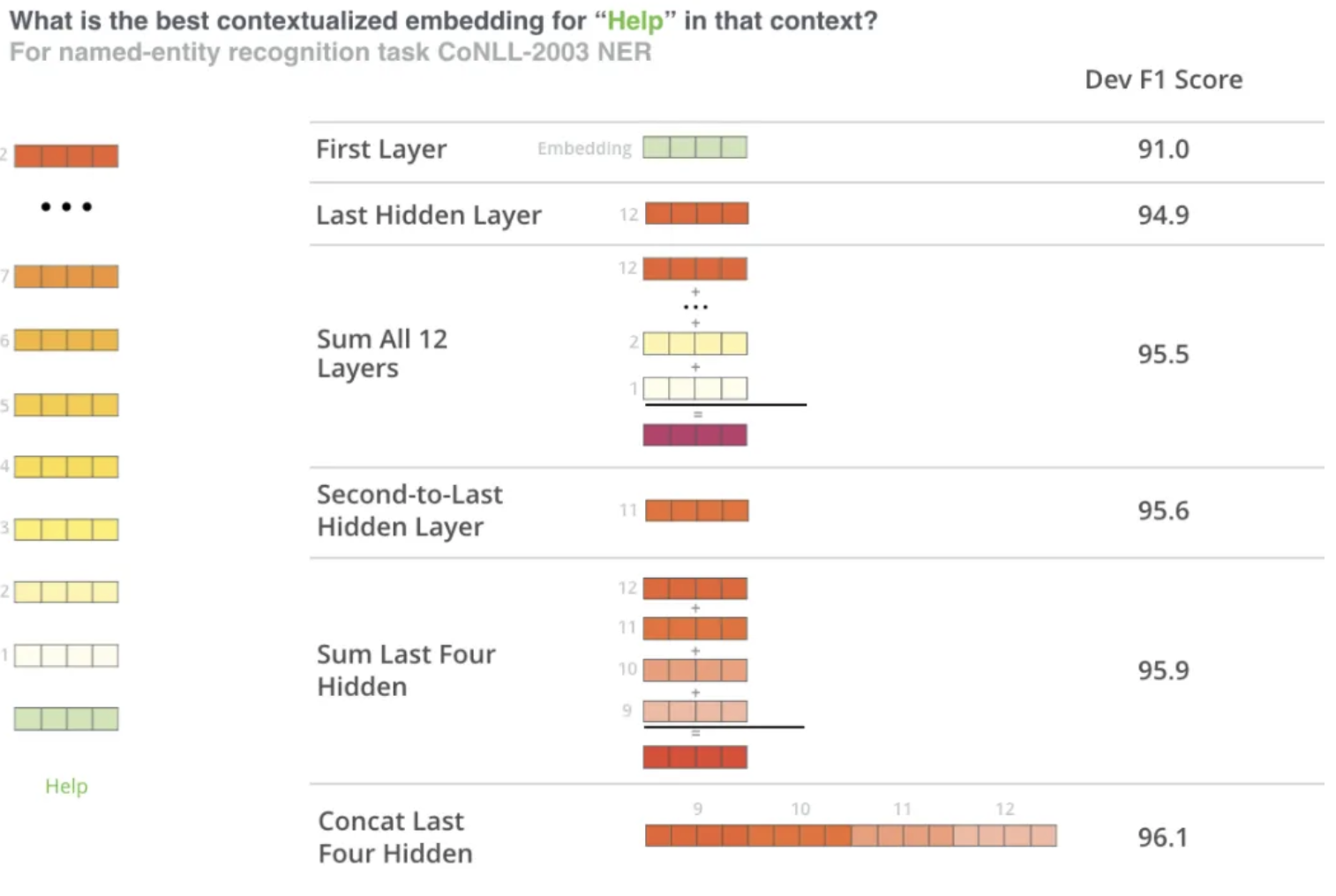
Since BERT is an Encoder Only Model, it basically takes an input, runs it through multiple Encoders, and would send it through an output layer at the end - this output layer tyipcally isn't useful by itself for Word Embeddings, so you would need to go back through the hidden state values and aggregate these in some way to produce Word, Sentence, or Document embeddings

BERT Word Embeddings

• Another reference link
• Most use cases of word embeddings can come straight out of a pre-trained core BERT model
• You could send a single word through and it would most likely just be a representation of the WordPiece Embedding layer at the start
• If you send multiple words through (a sentence) then you could try and reconstruct each individual words new embedding that was altered from the self-attention layers
  • bank in the sentence the large and sandy river bank will be attended to, and ultimately different, from the countries central bank because it's surrounding context words are different!
  • Typically you would send through the sentence and then pull back each $T_i$, or some mixture of $H_{a, b}$ hidden states, for each $w_i$ and that would represent your finalized word embedding that was attended to / altered from contextual self-attention!
• 

BERT Embeddings Pseudo Code

• We'd need to load in the WordPiece Tokenizer
• Tokenize our sentence input into Word Pieces
  • Will have some words get split into tokens like embeddings -> [em, ###bed, ###ding, ###s]
• Load the pre-trained BERT model
  • Set the model to eval() mode since you do not want to go through updating the base models weights for inference time
• Get the token ID's for each of these tokens from the pre-trained BERT state file
• Create a segement embedding (can just be repeated 0's and 1's of same size as token embeddings) which represent what sentence these tokens are apart of
  • In this scenario to embed one sentence you will most likely just have all 0's in our segment embedding
• Pass the token and segment tensors through the BERT model
• It will output all of it's hidden layers - these include multiple dimensions:
  • The layer number (13 layers)
    • Input WordPiece embedding + 12 hidden layers
  • The batch number (1 sentence)
    • Used to batch together multiple sentences for inference, for now it's just 1
  • The word / token number (22 tokens in our sentence)
  • The hidden unit / feature number (768 features)
• Most people permute this output to get it in the order of [# tokens, # layers, # features]
  • From this you have 13 separate vectors of size 768 for each token $w_i$
• Once this is done you can just directly SUM, CONCAT, AVG, etc...some mixture of hidden layers together to get our final word embedding
• TODO: Why do the hidden states represent the word embeddings? These don't get updated for our words right? If you model an entire corpus why would sending 0, 1000, 4500 through as a list of token ID's give us any sort of information? If I send through 0, 1001, 4500 are things that different even though I might be discussing a completely different word?
• TODO: What do the hidden layers of a BERT model represent? They're optimized parameters for language modeling...how does that relate to word embeddings?

Why does this work?

• The embeddings start out in the first layer with 0 contextual representation in them - river bank and central bank are the same bank embedding
• As the embeddings move deeper and deeper into the network they pick up more contextual information
• As you approach the final layer you start to pick up information about the pre-trained BERTs tasks, MLM and NSP respectively
• BERT is setup well to encode information, but at the end of the day BERT is meant to predict missing words or next sentences

BERT Sentence Embeddings

• Taking the above example, the typical way to get sentence embeddings is to SUM or AVG the second to last hidden state for each token in the sentence to achieve a sentence embedding

User Embeddings

TODO: Outside of collab filtering, how do you get user embeddings? TLDR; How do you get meaningful representations of users?

Embeddings vs Autoencoder vs Variational Autoencoder

This question has come up in my own thoughts, and others have asked me - they all get to a relatively similar output of representing things into a compressed numeric format, but they all have different training objectives, use cases, and architectures - Autoencoders were created to reduce dimensionality, and Embeddings were created to represent, possibly dense items, into dense numeric representations

Embeddings

Description

• Embeddings are dense vector representations of objects (e.g., words, users, items) that capture their semantic or contextual meaning in a continuous vector space
• They are typically learned during the training of a neural network and can be static (pre-trained) or dynamic (contextual)

Use Cases

• Static Embeddings:
  • Pre-trained embeddings like Word2Vec or GloVe are used for tasks where the context does not change (e.g., word similarity tasks)
  • Example: Representing the word "bank" as a fixed vector regardless of its context
• Dynamic Embeddings:
  • Contextual embeddings like BERT or GPT are used for tasks where the meaning of the object depends on its context
  • Example: Representing "bank" differently in "river bank" vs. "central bank."

When to Use

• Use embeddings when you need a lightweight, efficient representation of objects for tasks like:
  • Search and retrieval (e.g., cosine similarity between query and document embeddings)
  • Recommendation systems (e.g., user-item embeddings)
  • Pre-trained embeddings for transfer learning

Autoencoder

Description

• An Autoencoder is a type of neural network designed for dimensionality reduction. It learns to encode input data into a compressed representation (embedding) in the hidden layer and then reconstructs the original input from this representation
  • It's typically used to represent sparse data into a more compact format
• The encoder compresses the input, and the decoder reconstructs it
• So what's the difference between an Autoencoder and Word2Vec?
  • Word2Vec doesn't get train input word to be reconstructed on the other side (outright) like an Autoencoder, instead it tries to predict surrounding words...therefore the end results are ultimately the same, but the training tasks are different

Use Cases

• Dimensionality Reduction:
  • Reducing high-dimensional data into a lower-dimensional embedding while preserving important features
  • Example: Compressing image data for visualization or clustering
• Static Embeddings:
  • The hidden layer of the Autoencoder can be used as a static embedding for the input data
  • Example: Representing user profiles or item features in a recommendation system

When to Use

• Use Autoencoders when:
  • You need static embeddings for structured data (e.g., tabular data, images)
  • The input and output are the same, and you want to reduce dimensionality
  • You do not need to generate new data points but only want a dense representation of existing data

Variational Autoencoder (VAE)

Description

• A Variational Autoencoder is an extension of the Autoencoder that introduces a probabilistic approach. Instead of encoding the input into a single deterministic vector, it encodes it into a distribution (mean and variance)
• The decoder samples from this distribution to reconstruct the input, allowing the generation of new data points

Use Cases

• Generative Models:
  • VAEs are used to generate new data points similar to the training data
  • Example: Generating new images, text, or user profiles
• Dynamic Embeddings:
  • The latent space of the VAE can be used to create embeddings that capture uncertainty or variability in the data
  • Example: Representing user preferences with variability for personalized recommendations

When to Use

• Use VAEs when:
  • You need to generate new data points (e.g., synthetic data generation, data augmentation)
  • You want embeddings that capture uncertainty or variability in the data
  • The task involves probabilistic modeling (e.g., anomaly detection, generative tasks)

Comparison and When to Choose

Technique	Static Embeddings	Dynamic Embeddings	Generative Tasks	Dimensionality Reduction
Embeddings	Yes	Yes	No	No
Autoencoder	Yes	No	No	Yes
Variational Autoencoder (VAE)	No	Yes	Yes	Yes
Word2Vec	Yes	No	No	No

Key Considerations

1. Static vs. Dynamic Embeddings:

   • Use Autoencoders or Word2Vec for static representations
   • Use BERT or some sort of Transformer model with Attention for dynamic embeddings

2. Dimensionality Reduction:

   • Use Autoencoders or VAEs when you need to reduce the dimensionality of high-dimensional data

3. Generative Tasks:

   • Use VAEs when you need to generate new data points or capture variability in the data

4. Lightweight Models:

   • Use Word2Vec for lightweight, static word embeddings

Vector Similarities + Lookup

Vector similarities are useful for comparing our final embeddings to others in search space

None of the below are actually useful in real life, as computing these for Top K is very inefficient - approximate Top K algorithms like Branch-and-Bound, Locality Sensitive Hashing, and FAISS clustering are used instead

you discuss all of that here

Quantization

Quantization

• Definition: Quantization is a technique used to reduce the size of vector representations (e.g., embeddings) while preserving their ability to compare similarity effectively
• How It Works:
  • It reduces the precision of the numerical values in the vector (e.g., from 32-bit floating-point to 8-bit integers)
  • This compression reduces memory usage and speeds up computations, especially for large-scale systems.
• Key Idea:
  • The goal is to maintain the relative distances or similarities between vectors in the embedding space, even after reducing their size
• Use Cases:
  • Approximate Nearest Neighbor Search: Quantized vectors are often used in libraries like FAISS to perform fast similarity searches
  • Edge Devices: Quantization is used to deploy machine learning models on devices with limited memory and computational power (e.g., mobile phones, IoT devices)
• Limitations:
  • Quantization introduces some loss of precision, which can slightly affect the accuracy of similarity comparisons

Sketching

TODO:

Feature Multiplexing

TODO:

Cosine

Cosine similarity will ultimately find the angle between 2 vectors $\text{cosine similarity}(A, B) = \frac{A \cdot B}{|A| |B|}$

• Where
  • $( A \cdot B )$ is the dot product of vectors $( A )$ and $( B )$.
  • $( |A| )$ and $( |B| )$ are the magnitudes (or Euclidean norms) of vectors $( A )$ and $( B )$
    • Therefore, magnitude has no effect on our measurement, and you only check angle between vectors
• Cosine similarity ranges from $[-1, 1]$ where:
  • 1 indicates they're overlapping and pointing in the exact same direction
  • 0 indicates they're fully orthonormal (right angle) with 0 overlap over any dimensions
  • -1 indicates they're pointing in exactly opposite directions

Dot

The Dot product is similar to the Cosine product, except it doens't ignore the magnitude

$dot(a, b) = \sum_{i=1}^v a_ib_i = {|A| |B|}cosine(a,b)$

Which basically means you just compare each item over each dimension. If $a, b$ are normalized then Dot is equivalent to Cosine

Euclidean

This is the typical distance in euclidean space

$euclidean(a, b) = [\sum_{i=1}^v (a_i \times b_i)^2]^{1/2}$

Here magnitude matters, and a smaller distance between vector end-points means a smaller overall distance metric

Topological Interpretations

Most of this comes from Yuan Meng Embeddings Post

There you see discussions of how embeddings, topologically, can be considered a injective one-to-one mapping that preserves properties of both metric spaces

you can also see that from a ML lense, embeddings represent dense numeric features in n-dimensional space

• Images can go to 3 colors x 256 pixels dimension using photo represenation on disk (this is just how photos are stored)
• Text can go from sentences to 256 dimension vectors in Word2Vec or BERT
• Text can go from address sentences to [lat, long] 2 dimensions - you cover this in Address Embeddings

The main point of all of this is that Embeddings equate to → topological properties are preserved - that's what allows the famous King - man + woman = Queen and France is to Paris as Germany is to Berlin

A random list of numbers is a numeric representation, but they are not Embeddings

One-hot encoding, kindof, preserves topolological properties, but all of the vectors end up being orthogonal to each other so you can't say category1 + category2 = 0.5category3...they're orthogonal! Typically you need to map these from OHE metric space to a lower dimensional metric space to get those properties out of it

Dual Encoder

Much of the discussion below this point stems from this Multimodal Blog

Dual encoders have a number of different use cases and interpretations - there's using multiple encoders that end up in similar embedding spaces so you can do comparisons - this is helpful in RAG or query-document comparisons

There are other encoder architectures that focus on different modalities so that you can compare text to images to audio

At the end of the day, all of these architectures are designed so you can do dot-product similarity searches in an embedding space

Query Document Retrieval

A dual encoder consists of two separate neural networks that encode two different sets of data into their respective embeddings

For example:

• RAG $\rarr$ Uses a query encoder and a document encoder
• Question Answer $\rarr$ Uses a question encoder and an answer encoder
• There are other comparisons like caption and image, audio and language classification, or image to OCR

At the end of all of these, the two inputs are transformed into embedding space(s) which allow us to do similarity searches to find ANN's

Two Tower Architecture

During training in something like Question-Answer, you would encode each of them separately and then train to maximize the similarity between the two, and minimize the similarity between others

This can utilize a Contrastive Learning approach if there's a way to create augmentions, or if you use n-pair loss, or simply using Cross-Entropy Loss over entire dataset can work too

In examples online it mostly utilizes Cross-Entropy Loss over entire answer dataset

Two Towers is useful so you can pre-compute candidates and do fast ANN lookup during inference. It also helps solve some modality issues, but that's also covered later in Fusion

During Inference and Serving, all you have to do is calculate embedding for an incoming query and it allows us to quickly find ANN neighbors in an index and return the top K to the client. All document embeddings can be pre-computed, so you only have 1/2 of compute need during inference

• Run a batch prediction job with a trained candidate tower to precompute embedding vectors for all candidates, attach NVIDIA GPU to accelerate computation
• Compress precomputed candidate embeddings to an ANN index optimized for low-latency retrieval; deploy index to an endpoint for serving
• Deploy trained query tower to an endpoint for converting queries to embeddings in real time, attach NVIDIA GPU to accelerate computation

Google came up with a novel compression algorithm that allows for better relevance, and faster speed, of retrievals which is known as ScaNN. This service is then fully managed by Google Vertex AI Matching Engine

• Distributed search tree for hierarchically organizing the embedding space. Each level of this tree is a clustering of the nodes at the next level down, where the final leaf-level is a clustering of our candidate embedding vectors
• Asymmetric hashing (AH) for fast dot product approximation algorithm used to score similarity between a query vector and the search tree nodes

These architectures also allow us to address cold start problems since you can put through user features or generic default features to pull popular candidates

Multimodal Retrieval

Multimodal retrieval can be viewed as a specific implementation of Two Tower, where towers have different modalities - one may be a text query, and the candidates may be audio tracks

you can also use Fusion in our towers here so that whether it's a text or audio input you can use it and compare to image candidates for ANN lookup

Image2Text

This model focuses on image captioning or overall providing descriptive text for given images

It was one of the initial approaches to multi modality focusing on NLP and CV architectures that were combined into a shared embedding space

Microsofts Common Objects in Context (MS COCO) was a foundational dataset for this - it focuses on detecting non-iconic views, detecting semantic relationships between objects, and determining the precise localization of objects. It contained 91 common object categories with 328,000 images and 2.5 Million instance labels

Some Transformer architectures were used where the transformer consists of an encoder with a stack of self-attention and feed-forward layers, and a decoder which uses (masked) self-attention on words and cross-attention over the output of the last encoder layer

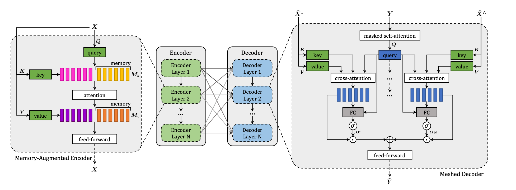
Ultimately it's a way for us to use Vision Transformers and Lanugage Encoders in the same model - one of the more useful examples was the Meshed-Memory Transformer for Image Captioning. The input was a photo with bounding boxes, and the image would get chunked out into a sequence and encoded with full self-attention. At the end each encoding layer output is fed into each decoder layer in a mesh-style relationship between the two layers

CLIP

Contrastive Language Image Pretraining (CLIP) is a transformer like architecture that jointly pre-trains a text encoder and an image encoder at the same time using Contrastive Learning

The contrastive goal is to correctly predict which natural language text pertains to which image inside a certain batch - this turned out to be more efficient than training on captions of images

Introduction to Fusion

Fusion involves combining multiple modalities into single models / architectures to aid in multimodal retrieval

It allows us to bypass model-per-modality - while this sounds like it can rid of two towers that's beside the point. Two Towers is useful so you can pre-compute candidates and do fast ANN lookup during inference

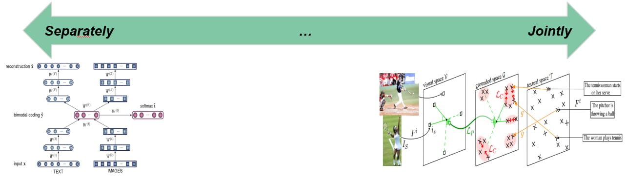
How to integrate multiple modalities? On one side of the spectrum, textual elements and visual ones are learned separately and then “combined” afterwards (left), whereas on the other side, the learning of textual and visual features takes place simultaneously/jointly (right)

The ultimate goal, that seems to have been achieved, is to move away from model-per-modality and focus on robust foundational models that can incorporate all types of modalities while allowing them to attend to each other

Some of the earliest movers were Data2Vec, Flamingo, and Vilbert - Data2Vec, for example, was to predict latent representations of full input data based on a masked view of the input in a self distillation step. you can see the parallels here between Transformers, Contrastive Learning, and Multimodality