CNN - ResNet and DenseNet
CNN Background
CNN's work well on image data - typical NN's will take an image, flatten it, and just pass it through a network. This is fine, but it doesn't generalize well across objects inside of images. Typical NN's aren't translationally invariant, but CNN's are!
Translational Invariance
Translational invariance is the property of a system that remains unchanged when its position or input data is shifted in space. It's important because generally we're more interested in the presence of a feature versus where it's actually at - once a CNN is trained to detect things in an image, changing the position of that thing in an image won't prevent the CNN's ability to detect it
CNN Layers
There are multiple layer types in CNN's that are discussed elsewhere:
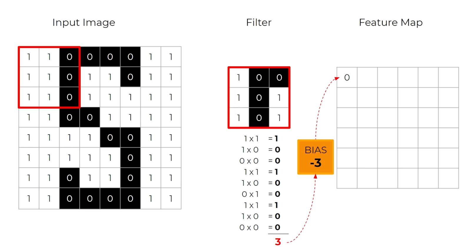
- Convolutional layers take sliding windows (filters / kernels) over pixels to extract local features like edges and textures. Each filter produces a feature map by aggregating pixels in it's window
- Pooling layers will reduce the actual spatial size of feature maps by sliding a window and applying an aggregate function (max, avg, etc) to that region
- Dense layers (fully connected layers) have each neuron connected to another next layers neurons, and these are for combining features from above layers
- Activation layers look to take these other layers and look for features by utilizing non-linear functions such as ReLU, sigmoid, tanh, etc to introduce non-linearity inside of the network
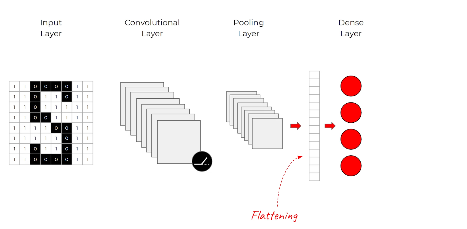
Instead of flattening inputs, CNN's apply filters by utilizing convolutional and pooling layers. These filters stride over the entire input image or hidden layers
ReLU layers also allow CNN's to find edges, textures, etc because color gradients will change from -1 to 0 and other features, and pooling layers inbetween help reduce the size of the problem space as it grows. All of this ends up being passed into final softmax layers and other things to predict image classes, output bounding boxes, etc.
ResNets
Learning better networks isn't as easy as just simply stacking more and more of those above layers on! Unlike NLP, where more attention layers allow for better embedding representations, CNN's showed diminishing returns and sometimes complete degredation when stacking more of these layers together
ResNets were presented as an answer to "can stacking more layers enable the network to learn better" - the obstacle up to that point was vanishing / exploding gradients, and they were primarily solved for by normalized initialization and intermediate normalization layers which enabled networks with tens of layers to start converging for stochastic gradient descent with backprop. Degredation also proved to be an issue, where as network depth increased there was a saturation, and then rapid decrease, in accuracy. Adding more layers to a suitably deep model led to higher training error, and overfitting was not caused by this degredation. A shallower architecture was suggested, and using auxiliary layers consisting of identity mappings and others shallow model layers, but in practice this didn't help. Later on Deep Residual Learning took the charge, and utilized normalization / residual layers to help fix the problems of degredation
Parameters early on in CNN architectures sometimes don't receive meaningful gradient updates (vanishing gradients), sometimes the gradients are huge and chaotic (exploding gradients), the layers may not capture meaningful representations (just bad NN), or extra layers may degrade useful features in hidden layers (degredation)
ResNets are an architecture that show promise in fixing many of the above issues, ultimately preserving gradients and allowing features to pass through downstream layers
ResNet Theory / Background
ResNet Architecture
Deep Residual Learning
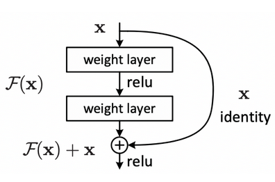
Deep Residual Learning is useful in the ResNet sense because it allows very deep networks to be trained by reformulating the layers as learning residual functions with reference to the layer inputs, rather than directly learning unreferenced functions. This helps address the vanishing gradient problem and enables effective training of much deeper architectures
There was a huge issue of exploding / vanishing gradients, along with overall degredation of accuracy in these models, that were solved by utilizing normalization layers and residuals - ResNets usage of residual skip conncetions specifically addresses the degredation problems
The degredation problem ultimately motivated the usage of residual learning
- In theory, if you add more layers to a NN the network should be able to at least match the performance of a shallower network, simply by learning the identity function
- i.e. the extra layers don't actually do anything
- In practice, deep networks often perform worse (measured by a higher training error) as more layers were added - this is the degredation problem
- The reason for this problem is that it's surprisingly hard for standard (non-residual) deep networks to learn the identity mapping using many non-linear layers. Ultimately the optimization process just can't find this solution
- Residual learning re-formulates the problem
- Instead of learning , some full mapping
- It aims to learn the residual
- So
- Why?
- If the best thing for the extra layers to do is nothing (identity function of shallow network), the residual can just go to zero, which is easier for an optimizer to find
- If the optimal function is not an identity function, it's often closer to identity thatn zero, so learning a small "perturbation" from identity is easier for the optimization to learn instead of doing it from scratch
- If the optimal function starts to converge to a non-zero solution, then the middle mapping layers can be considered worthwhile, as they add some sort of new information
- Altogether, Residual connections make it easier for deep networks to learn functions that are closer to identity mappings, which help to avoid the degredation problem and make optimization easier
This entire thought process created the problem statement for residual learning frameworks / layers inside deep NN's.
Residual Learning
The idea of residual learning is to replace the approximation of an underlying latent mapping , which is approximated by a few stacked layers, with an approximation of residual functions where denotes the inputs to the first of these few stacked layers - therefore
Below, the is the residual mapping that is to be learned, an example is in which denotes the ReLU activation function - most experiments show that ID mapping is enough to solve the degradation problem
EfficientNet
Before EfficientNet it was popular to scale only one of three dimensions - depth, width, or image size. Research papers and empirical studies, which ultimately led to EfficientNet, showed it's critical to balance all dimensions which can be achieved by scaling all 3 with a consistent ratio.
Compound Model Scaling
A function with operator , output tensor , and input tensor of shape spatial dimensions and channel dimension is called a ConvNet Layer i
A ConvNet appears as a list of these composing layers
Effectively, these layers are often split / partitioned into multiple stages and all layers in each stage share the same architecture - an example is ResNet which has 5 stages (), with all layers in each stage being the same convolutional type except the first layer which performs down-sampling.
Scaling all 3 is important as they'r all fairly linked - you cannot increase the resolution of an image without increasing it's depth and saturation (idk what this means). Therefore, a compound scaling method which uniformly scales network width, depth, and resolution is required
Contrastive Learning
We've looked into Contrastive Learning in another sub-document, and will copy this section over there, but this is a section specifically on Image based Contrastive Learning
SlimCLR was one of the first, and most known, contrastive learning frameworks - it's simple, highly accurate, well researched, and heavily utilized. The main idea is to have two copies of a single image, and use these to train two networks that are compared. A major con is that it doubls the overall storage size of the underlying dataset, but BLOB storage is cheap (in my opinion). Boostrap Your Own Latent was introduced to avoid making the double sized dataset.
Contrastive Learning Framework
Contrastive loss is used to learn a representation by maximizing the agreement between various augmented views of the same data example. To achieve this, there are 4 significant components:
- A stochastic data augmentation module to create new augmentations of input
- A neural network base encoder to take inputs, and augmentations, and will encode into dense vector
- A small neural network projection head to take encoded vectors into projection space
- A contrastive loss function that allows comparisons between projected vectors

Stochastic Data Augmentation
A minibatch of examples is sampled randomly, and thee contrastive prediction task is defined on pairs of augmented examples - this results in data points altogether
A memory bank isn't needed, as the training batch size varies from 256 to 8,192. Any given data example randomly returns two correlated views of the same example, denoted as and which is known as the positive pair. The negative pair are all other pairs. It's been shown that choosing different data augmentation techniques can reduce the complexity of previous contrastive learning frameworks. Some of the common ones are:
- Spatial geometric transformations like cropping, resizing, roration, and cutouts
- Appearance transformations like color distortion, brightness, contrast, saturation, Gaussian blur, or Sorbel filtering
Models tend to improve after composing augmentaitons together too, instead of only applying one single one
Neural Network Base Encoder
The NN Base Encoder extracts multiple representation vectors from the augmented data examples - the commonly used ResNet was picked and gives where is the output after the average pooling layer.
Small Neural Network Projection Head
A small neural network projection head maps the representation to the space where the contrastive loss is applied. The importance of this layer was evaluated with:
- Identity mapping
- Linear projection
- Default non-linear projection with an additional hidden layer and ReLU activation
The results showed the non-linear projection is better than linear, and both are much better than no transformation (identity)
They've used an MLP with one hidden layer to obtain where is a ReLU non-linear transformation
This is useful because defining the contrastive loss on instead of wouldn't lead to a loss of information caused by contrastive loss, and is shown to maintain and form more information
Contrastive Loss Function
Given a set including a positive pair of examples and , the contrastive prediction task aims to idntify in for a given . In the case of positive esxamples, the loss function is defined as
Where:
- is the loss for the pair
- is the similarity between and
- Typically is a dot product between and normalized
- is the temperature parameter
- is the indicator function (1 if , 0 otherwise)
The final loss is calculated across all positive pairs, both and in a mini-batch
This above was named NT-Xent as Normalized Temperature-scaled Cross Entropy. This was compared against other commonly used contrastive loss functions like logistic loss and margin loss, and NT-Xent outperformed with proper hyperparameter tuning
SlimCLR Framework
The ultimate goal of this framework was to describe a better approach to learning visual representations without human supervision.
SlimCLR outperforms previous work, is more straightforward, and does not require a memory banks
Significant components of the framework:
- A constrastive prediction task requires combining multiple data augmentation operations, which results in effective representations
- Unsupervised contrastive learning benefits from more significant data augmentation
- In english, this means applying lots of different random changes (like cropping, flipping, rotating, color changes, etc) to images. The model is trained to recognize that these different augmentations are "the same"
- The quality of learned representations can be substantially improved by introducing a learnable non-linear transformation between the representation and contrastive loss
- Basically this means you encourage the model to make the representations (feature vectors) of different augmented views of the same image similar, while making representations of different images dissimilar
- Contrastive loss will penalize the model is the two feature vectors of the same augmented image are far apart, and rewards them if they're similar
- Common contrastive loss example is NT-Xent (Normalized Temperature-scaled Cross Entropy) loss
- Representation learning with cross-entropy loss can be improved by normalizing embeddings and adjusting the temperature parameter appropriately
- Temperature is a parameter in the contrastive loss function that controls how sharply the model distinguishes between similar and dissimilar pairs
- A lower temperature makes the model focus more on making positive pairs very close, and negative very far apart
- A higher temperature smooths out the differences, making the model less strict about separating pairs
- Therefore, this equates to saying that adjusting the temperature to balance how hard the model pushes similar images together can improve the quality of the learned representations
- Temperature is a parameter in the contrastive loss function that controls how sharply the model distinguishes between similar and dissimilar pairs
- Contrastive learning benefits from larger batch size and extended training periods compared to supervised counterpart
- Larger batch size helps because it allows the model to compare more positives and negatives for each sample
- Each batch is used to create positive and negative pairs, so the more examples inside of it the more comparisons!