Loss Functions

Output Layers

The final output layers of our models typically go hand-in-hand with the Loss Functions that you use

Regression

Regression output layers are used when the task is to predict continuous values

Linear

• Usage: Regression
• Description: The linear output layer outputs a continuous value. It is used for regression tasks where the goal is to predict a continuous variable
• Formula: $[ y = w \cdot x + b ]$
• Where:
  • $( y )$ is the predicted output
  • $( w )$ is the weight matrix
  • $( x )$ is the input vector
  • $( b )$ is the bias term

Classification

Classification output layers are used when the task is to predict discrete labels or categories

Why do you use these output formulas? you want them to be "nice" for derivates and not to have vanishing gradients. They're also fairly intuitive for each of the specific tasks they're used for.

Sigmoid

• Usage: Binary classification
• Description: The sigmoid function outputs a probability value between 0 and 1 for each class. It is typically used for binary classification tasks
• Formula: $\sigma(x) = \frac{1}{1 + e^{-x}}$

Softmax

• Usage: Multi-class classification
• Description: The softmax function outputs a probability distribution over multiple classes. It is used for multi-class classification tasks
• Formula: $\text{softmax}(x_i) = \frac{e^{x_i}}{\sum_{j} e^{x_j}}$

Other Types

Log Odds, Logit, Logistic, Etc

Odds are just the probability of success over probability of failure $P \over {1 - P}$

Probability and odds are just 2 ways of formalizing the way to view chances, and in some cases like Logistic Regression log-odds are used simply because it's easier than dragging around a bunch of exponentials and logs.

Log-Odds has some useful properties that just make it a useful function similar to Sigmoid and ReLU

Logs Refresher

Logs are an alternative way to express exponents in terms of the end-result of applying an exponent to a number - therefore something like $\log_{20}(400)$ means "how many times do you need to multiple 20 by itself until you get 400"

It just gives us the total number of operations needed, but it also takes a multiplicative thing (multiplying by yourself in an exponent) and turns it into additive.

Outside of this, there are properties of logs that enable it to be used as a function that you can "undo" - i.e. if you have some numbers, convert to logs, and use below properties to transform it, you can then undo the log part and get to the expected outcome

• Quotient rule: $\log({M \over N}) = \log(M) - \log(N)$
• Product rule: $\log({M \cdot N}) = \log(M) + \log(N)$
• Power rule: $\log({M^N}) = \N \cdot log(M)$

Using Logs With Odds

Logs help to get rid of the non-intuitive nature of odds - mostly around reciprocals, interpretation, and symmetry

If the probability of success of an experiment $P$ is 40%, then

• Odds of success would be ${4 \over 6} = .667$
• Odds of failing are ${6 \over 4} = 1.5$

There isn't any good symmetry between the odds of success and failure, and increasing or decreasing $P$ isn't intiutively going to change the odds in a straightforward way

Logs help to fix that:

• $\log({4 \over 6}) = \log(4) - \log(6) = -.405$
• $\log({6 \over 4}) = \log(6) - \log(4) = .405$

Which shows how the symmetrical side of odds now

Logit

Logit formalizes what the log-odds look like for any conceivable set of odds - formally Logit function maps the probability of an event $P$ to its log-odds

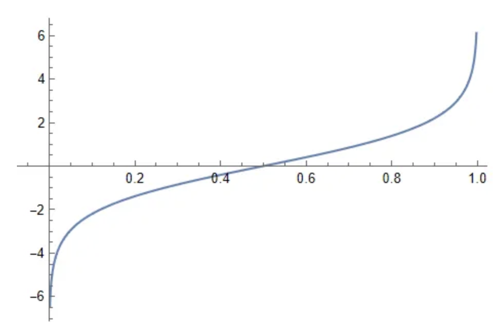
The Logit function is the inverse of the standard Logistic Distributions Cumulative Distribution function, aka quantile function of standard logistic distribution

• Quantile Function: Maps the probability values for a given distribution to the value of the random variable that would make the below statement true:
  • The random variable falls at or below $y$ with probability $x$
• Cumulative Distribution Function: The quantile function for any distribution is the inverse of the Cumulative Distribution Function (CDF) associated with the distribution. CDF's map the values of a random variable producing the distribution to the probability that makes the following statement below true:
  • The random variable falls at or below $x$ with probability $y$
• Therefore, quantile and CDF functions just give a way to view / interrogate a distribution in different ways
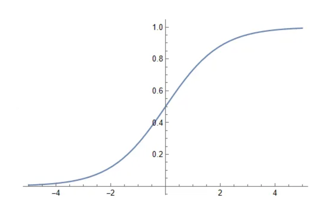
  • Logistic Distribution is a CDF, and the logit is a quantile function

Logistic Distributions

Logistic distributions are good for approximating a process that grows exponentially, but is ultimately capped by some limiting reason. The values grow quickly at first and eventually reach a limit

Softmax with Temperature

• Usage: Multi-class classification with control over the confidence of predictions
• Description: The softmax with temperature function introduces a temperature parameter to control the confidence of the predictions. Lower temperatures make the model more confident, while higher temperatures make it less confident
• Formula: $\text{softmax}(x_i, T) = \frac{e^{x_i / T}}{\sum_{j} e^{x_j / T}}$

Logits

• Usage: Intermediate representation for classification
• Description: Logits are the raw, unnormalized scores output by the model before applying a softmax or sigmoid function. They are often used as an intermediate representation in classification tasks

Tanh

• Usage: Regression or binary classification
• Description: The tanh function outputs values between -1 and 1. It can be used for regression tasks or binary classification tasks where the output needs to be in this range
• Formula: $\tanh(x) = \frac{e^x - e^{-x}}{e^x + e^{-x}}$

Loss Functions

Loss functions are the entire heart of model training and tuning

Log-Likelihood / Negative Log-Likelihood

Log-likelihood is a foundational concept in statistical modeling and machine learning. It measures how probable the observed data is under a given model and set of parameters. In practice, you often use the negative log-likelihood (NLL) as a loss function, since minimizing NLL is equivalent to maximizing the likelihood of the data.

Formula

$\mathcal{L}_{\text{NLL}} = -\sum_{i} \log p(y_i | x_i, \theta)$ Where:

• $p(y_i | x_i, \theta)$ is the probability assigned by the model to the true label $y_i$ given input $x_i$ and parameters $\theta$.

Use Cases

• Likelihood Estimators: Maximum Likelihood Estimation (MLE) uses log-likelihood to find the best model parameters.
• Bayesian Outputs: In Bayesian models, the likelihood is combined with a prior to form the posterior; log-likelihood is central to Bayesian inference and model comparison.
• General ML Topics: Log-likelihood is the basis for many loss functions (e.g., cross-entropy for classification, Gaussian NLL for regression) and is used in probabilistic models, generative models, and unsupervised learning.

Cross Entropy

Cross Entropy is a loss function commonly used for classification tasks. It measures the difference between the true probability distribution (ground truth) and the predicted probability distribution (output of the model)

It is particularly effective when the output of the model is a probability distribution (e.g., from a softmax layer)

Formula

$H(p, q) = -\sum_{i} p_i \log(q_i)$ Where:

• $p_i$: True probability of class $i$ (ground truth, typically one-hot encoded).
• $q_i$: Predicted probability of class $i$ (output of the model).

Use Cases

• Binary Classification:
  • Used with a sigmoid activation function for tasks with two classes (e.g., spam vs. not spam).
  • Example: Predicting whether an email is spam or not.
• Multi-Class Classification:
  • Used with a softmax activation function for tasks with more than two classes (e.g., classifying images into categories).
  • Example: Classifying images into categories like cats, dogs, and birds.

Why Use Cross Entropy?

• Penalizes incorrect predictions more heavily when the model is confident but wrong.
• Works well when the output is a probability distribution, as it directly compares the predicted probabilities to the true probabilities.

---

L2 Loss

TODO: L2

Log Likelihood

KL Divergence

KL Divergence (Kullback-Leibler Divergence) is a measure of how one probability distribution $q$ (predicted) diverges from a second probability distribution $p$ (true). It is often used in tasks where the true labels are probability distributions rather than one-hot encoded labels.

Formula

$D_{KL}(p \| q) = \sum_{i} p_i \log\left(\frac{p_i}{q_i}\right)$ Where:

• $p_i$: True probability of class $i$ (ground truth distribution).
• $q_i$: Predicted probability of class $i$ (output of the model).

Use Cases

• Probabilistic Outputs:
  • Used when the ground truth is a probability distribution (not one-hot encoded).
  • Example: Language modeling tasks where the ground truth is a smoothed probability distribution over words.
• Regularization:
  • Often used as a regularization term in models like Variational Autoencoders (VAEs) to ensure that the learned latent distribution is close to a prior distribution (e.g., Gaussian).

Why Use KL Divergence?

• Useful for comparing two probability distributions rather than a single label.
• Penalizes predictions that deviate significantly from the true distribution.

---

When to Use Cross Entropy vs. KL Divergence

Scenario	Use Cross Entropy	Use KL Divergence
Binary Classification	Use Cross Entropy with a sigmoid activation function.	Not applicable.
Multi-Class Classification	Use Cross Entropy with a softmax activation function.	Not applicable.
Ground Truth is a Probability Distribution	Not applicable.	Use KL Divergence to compare the predicted and true distributions.
Language Modeling	Use Cross Entropy when the ground truth is one-hot encoded.	Use KL Divergence when the ground truth is a smoothed or probabilistic distribution.
Regularization	Not applicable.	Use KL Divergence to regularize the predicted distribution (e.g., in VAEs).

Example Scenarios

1. Image Classification:

   • Task: Classify images into categories (e.g., cats, dogs, birds).
   • Use Cross Entropy with a softmax activation function, as the ground truth is one-hot encoded.

2. Language Modeling:

   • Task: Predict the next word in a sentence.
   • Use Cross Entropy if the ground truth is one-hot encoded (e.g., the next word).
   • Use KL Divergence if the ground truth is a smoothed probability distribution over words.

3. Variational Autoencoders (VAEs):

   • Task: Learn a latent representation of data.
   • Use KL Divergence to regularize the latent distribution to match a prior (e.g., Gaussian).

4. Recommendation Systems:

   • Task: Predict the probability of a user interacting with an item.
   • Use Cross Entropy if the ground truth is binary (e.g., clicked or not clicked).
   • Use KL Divergence if the ground truth is a probability distribution over items.

InfoNCE Loss

InfoNCE loss, or Information Noise-Contrastive Estimation loss is used in self-supervised learning, particularly Constrastive Learning to train models to learn meaningful representations by distinguishing between positive and negative sample pairs

During self-supervised contrastive learning you take an input data point and augment it with multiple functions to create multiple positive pairs, and then you can compare those with other samples which act as negative pairs

It does this by giving low loss to similar pairs - i.e. by maximizing the similarity between positive pairs, and minimizing the similarity between negative pairs

The key idea / intuition is to treat the learning problem as a binary classifier, where the similarity between instances is measured using a probabilistic approach - similar to Softmax

Formal Definition

Given a set $X = \{x_1, x_2, ..., x_N\}$ of $N$ random samples containing one positive sample from $p(x_{t+k} | c_t)$ and $N-1$ negative samples from the 'proposal' distribution $p(x_{t+k})$, you optimize:

$\mathcal{L}_{\text{InfoNCE}} = -\mathbb{E} \left[ \log \frac{\exp(\text{sim}(z, z^+)/\tau)}{\exp(\text{sim}(z, z^+)/\tau) + \sum_{j=1}^{N-1} \exp(\text{sim}(z, z_j^-)/\tau)} \right]$

Weight Updating

How to actually update weights from output of loss function

Gradient Descent

Gradient Descent is the main algorithm for updating weights based on our loss functions - it will basically chain together a bunch of partial derivatives which show each parameters effects on the output, and based on the output's loss the weights will be updated in the negative direction

It's simply a way to move parameters towards places that create "good" layers to create the final output layer as close as possible to what we're trying to model

Gradient Descent will run over all training examples