Evaluation Frameworks

Evaluation Frameworks

Evaluation is at the heart of all things ML - it's very easy to spin up models and run .predict(), but a majority of actual ML systems entirely start from evaluation and metrics

Every successful ML project I've been apart of has had metrics for evaluation, there are some projects that have had them which have been unsuccessful, but because of metrics it was apparent right away and the projects closed out quickly

Every project without metrics is unsuccessful (hyperbole, but still mostly true) because even if the model truly works how can you quantify it's abilities to anyone? If everyone has faith in you then maybe it'll work

There are a number of ways to evaluate ML systems, and most start with Offline Metrics which are able to be calculated using large aggregate queries and ground truth labels, and are typically tailored to "measuring accuracy". Online Metrics require systems to be up and running with actual feedback from users, and are typically tailored to "influence and abilities"

A majority of the metrics in Online vs Offline are based on metrics for Candidate Generation, and [Ranking], which revolve around "recommended lists", and then there are other metrics below for [Regression] along then Loss Functions are covered in a completely different document

Most of these are just useful to convery in this setup, but it doesn't mean each metric can't be used elsewhere

Stages

There are multiple stages that are included for most of these things, and some of the stages will change with different systems

• In something like generic binary classifier you only have training + evaluation stages, and it's not very complicated
• In other systems like Recommender Systems, you will have
  • Stages:
    • Candidate Generation
    • Ranking
    • Maybe Re-Ranking
    • Final Serving
  • Each of these stages focus on differnet areas and metrics - in Candidate Generation you'd want to focus on Recall and "for any potential match, we want to ensure we include it, and we may include bad matches" which equates to high recall and lower precision
  • Afterwards, in steps like Ranking and Re-Ranking you whittle down the result set to increase Precision and include business rules
    • Ranking may just be a supervised model based on historic data, and Precision here may be different than with business rules that want to increase certain products during promotions
      • It's harder to keep seasonal product rotations in a validation set, so this may be evaluated differently

So in the rest of this article, we'll focus on more complicated RecSys and Entity Resolution type topics because they tend to cover the rest of the universe to some extent

Online Vs Offline

As stated above, Offline Metrics are able to be calculated using large aggregate queries and ground truth labels, and are typically tailored to "measuring accuracy" whereas Online Metrics require systems to be up and running with actual feedback from users, and are typically tailored to "influence and abilities"

Offline Evaluation

Offline metrics and testing is most often used as a pre-production testing setup to ensure our model performs well on new data and hasn't regressed / become worse

Outside of that, these metrics also help us in hyperparameter tuning and experimentation to tweak parameters / business rules and see the effects

Typically, offline metrics revolve around calculating accuracy metrics like

• $Precision = {{TP} \over {TP + FP}}$
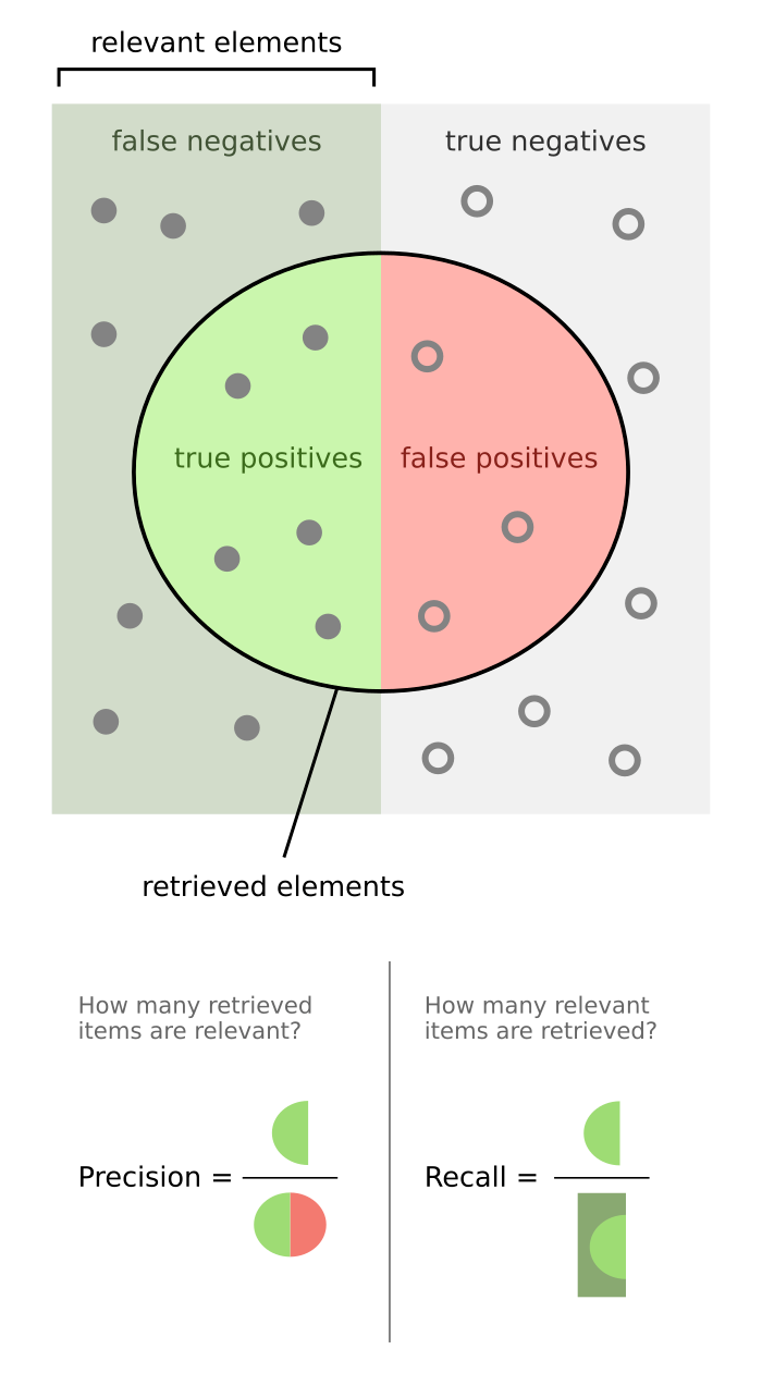
  • It can be viewed as "Out of everything that was recommended, what was actually relevant?"
  • It is # of recommended items that are relevant over total number of recommended items
    • ${TP + FP}$ comes out to be all recommended items

  ---

• $Recall = {{TP} \over {TP + FN}}$
  • It can be viewed as "out of everything that should have been recommended, what was?"
  • It is number of # of recommended items that are relevant over total number of relevant items
    • ${TP + FN}$ comes out to be all relevant items

  ---

• $F_1 = \frac{2 \cdot TP}{2 \cdot TP + FP + FN}$
  • F1 will end up combining all aspects of precision / recall matrix to calculate a more comprehensive score (weighted towards true positives)

  ---

• Log-Likelihood
  • Measures the goodness of fit of a model by calculating the logarithm of likelihood function
  • It's typically used in latent factor models, and can be used to score the log-likelihood of observing the user-item interactions given the models parameters
  • Log-likelihood as a whole is a broad stats / ML topic that is used in quantifying parameters "likelihood"

---

There are other more advanced metrics that involve ranking such as:

• @k Metrics
  • $Precision@k = {{(TP)@k} \over {(TP + FP)}@k}$
  • $Recall@k = {{(TP)@k} \over {TP + FN}}$
    • Notice Recall@k still has a denominator over the entire dataset, because Recall@k measures the completeness of the retrieved set relative to all existing relevant items
    • Precision@k just asks "out of everything we recommended, what % is relevant" so it's denominator is at the k-subset level
  • @k Metrics will score the above metrics up to a certain # of recommended items, $k$
    • Some of this will utilize position in the ranking, and some won't - the idea being that we penalize systems if all of the desired recommendations are at the bottom of the final output list!
    • The @k calculations will loop over $[1, 2, ... , k]$ and calculate precision and recall, thus including some sort of ordering penalization in the scores
      • If your results are stored in $[k - 3, k]$ instead of $[1, 2, 3]$, your scores will be worse, thus it includes some order
      • These do not strictly enforce an item is at position $i$ is better than an item at position $i+1$, it simply ensures the items are in some list
  • These metrics also help when our viewport size is different, a laptop can usually display more items than a phone
  • $\text{Average Precision@k}$ and $\text{Average Recall@k}$ will run precision and recall over a sliding window of top-k results, and then compute the average over sliding window of truly relevant results in there
    • For different devices / potential k's, this would change and allow us to compare different environments
  • $\text{Average Precision@k} = {{\text{Precision@1} + \text{Precision@2} + ... \text{Precision@k}} \over {TP + FN}}$
    • Where ${TP + FN}$ is the number of relevant items in the top-k results for a query
    • For query $q$: $AP@k = \frac{1}{\min(m, k)} \sum_{i=1}^{k} P(i) \cdot rel(i)$
      • $m$ = total number of relevant items for $q$
      • $P(i)$ = precision at position $i$
      • $rel(i)$ = 1 if item at position $i$ is relevant, 0 otherwise
    • The above is an easier calculation to run over large datasets
  • $\text{Average Recall@k} = {{\text{Recall@1} + \text{Recall@2} + ... \text{Recall@k}} \over {TP + FN}}$
  • A good article for these 2
  • $\text{Mean Average Precision MAP@k}$ and $\text{Mean Average Recall MAR@k}$ will then take the equations above and average them across all users
    • These allow us to gauge aggregated measures of recommender systems performance across positions, users, and environments
  • Both MAP and MAR are both designed for binary relevance judgements where an element is relevant or not
    • If there are sliding scales of relevance, the ideal metric is Normalized Discounted Cumulative Gain
    • 

  ---

• $\text{Fraction of Concordant Pairs (FCP)} = {{NCP} \over (NCP + NDP)}$
  • $NCP$ = # of concordant pairs, which are pairs whose ranking is consistent with user preferences
    • A pair $(i, j)$ is concordant if the user prefers $i$ over $j$ by way of click-preference, view time, or some other implicit/explicit feedback
    • Notice the relative rank only matters, meaning $i \gt j$, it doesn't care by how much
  • $NDP$ = # of disconcordant pairs, which are not consistent with user preferences
  • A ranking metric that evaluates how well a recommender orders items in alignment with user preferences
  • FCP focuses on pairwise correctness of rankings, and provides a measure of ranking quality by comparing relative positions of items
  • $range \in [0,1]$ where $1$ means perfectly concordant
  • Limitations:
    • Has quadratic growth given every pair in user preferences is compared to every other pair
    • Computationally expensive to compute for each batch
    • Relies heavily on well-defined user data gathering and preferences between pairs of items, which may not be obtainable

  ---

• $\text{Mean Reciprocal Rank (MRR)} = { {1 \over m} \cdot \sum_{i=1}^{m}{1 \over \text{rank}_i}}$
  • $m$ is the total number of output lists (# of users / queries)
  • $\text{rank}_i$ denotes the position of the first relevant item in the $i^{th}$ output list
  • Particularly useful in scenarios where explicit relevance labels are unavailable
    • In this case, a system would rely on implicit signals like user clicks or interactions
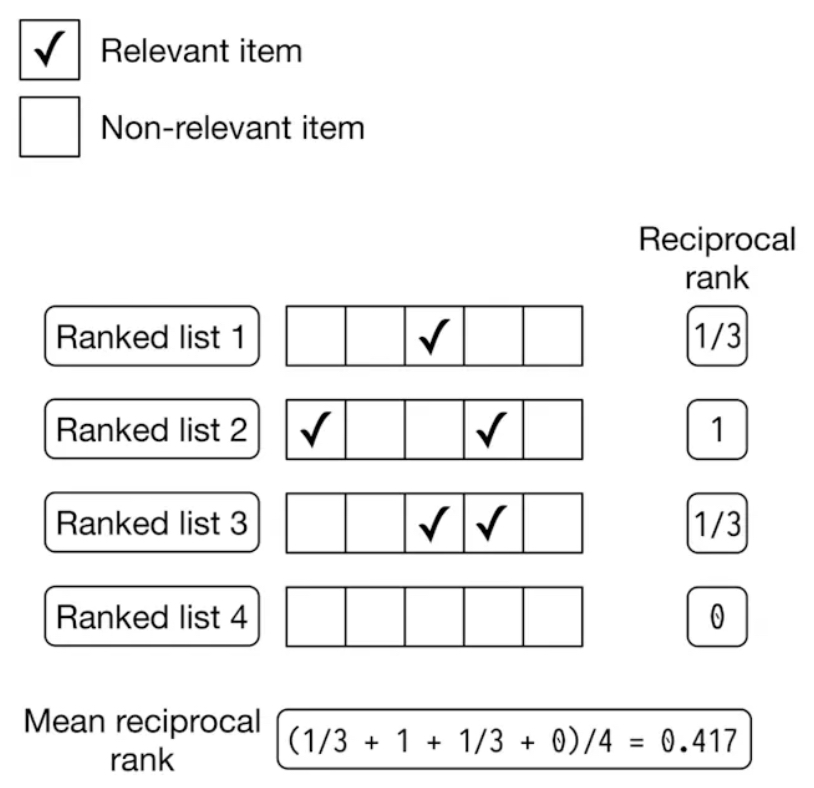
  • MRR considers the position of the recommended items when determining relevance, and ultimately MRR quantifies how effectively an algorithm ranks the correct item within a list of recommendations
  • $\text{Reciprocal Rank (RR)} = {1 \over \text{rank}_i}$
    • Therefore, a mean reciprocal rank is going to be the average RR across all queries and users
    • MRR evaluates quality of a model by considering the position (rank) of first relevant item in each output list generated by the model
      • Across multiple users or multiple queries per user
    • Afterwards, it averages everything out
  • Limitations:
    • Only focuses on first relevant item, and not all items
  • 

  ---

• $\text{Average Reciprocal Hit Rate (ARHR)} = { {1 \over |U|} \cdot \sum_{u \in U} \sum_{i=1}^{k}{1 \over \text{rank}_i(u)}}$
  • ARHR is often used interchangeably with MRR
  • ARHR is a generalization of it, and is used in scenarios involving multiple clicked items
  • $\text{Reciprocal Hit Rate (RHR)}$ is computed for each user by summing reciprocal of the positions of the clicked items within the recommendation list
    • If $3^{rd}$ item is clicked, reciprocal would be $1 \over 3$
    • RHR is the sum of the reciprocals for every item for a user
  • ARHR is then averaging all of these across all users
• ARHR and MRR are both useful in ensuring the most relevant items (top) are showcased high up in the recommended list
  • Neither care much about placement of other relevant items

  ---

• $\text{Normalized Discounted Cumulative Gain (nDCG)} = {\text{DCG} \over \text{IDCG}}$
  • $\text{DCG}$ and $\text{IDCG}$ are discussed below after going through $\text{CG}$
  • nDCG is a list wide ranking metric commonly used to check quality of a list of recommendations
  • It allows us to go past binary "relevant or not", and utilize scores / percentages of relevancy
    • nDCG considers relevance on a continuous scale
  • nDCG requires a list that includes the ranking information for each relevant item
    • Idea is that items ranked higher should be more relevant, thereby contributing more significantly to overall quality of ranking
  • To understand nDCG we need to understand:
    • $\text{Discounted Cumulative Gain}_{p} = { \sum_{i=1}^{p} {\text{relevance}_{i} \over {\log_{2}(i + 1)}}}$
      • Discounting the Cumulative Gain calculation below means weighting each entry in the list based on its position in the list
        • If there's a highly relevant item in position $N$, and the rest from $[1, 2, ..., N-1]$ are basically irrelevant, we would not weight that differently from a list with the most relevant item in position 1
      • $i$ is the position of the item in the ranked list (starting at 1)
      • The discount is the $1 \over {\log_{2}(i + 1)}$ portion
        • $\log_{2}(i + 1)$ is the discounting factor
        • As $i$ becomes larger, we reduce the overall weight of the relevance score
      • $p$ is the position in the ranked list where you want to calculate DCG up to
        • If this is item $1$, $k$, or $N$ it doesn't matter, we can also do a sliding window and average if desired
          • This would be some metric like Mean-Discounted Cumulative Gain MDCG
      • $i$ is an output of the model (it's position in final ranking) and relevance is an output of labeling / user feedback - they are calculated at 2 different areas of the process
    • $\text{Cumulative Gain} = \sum_{i=1}^{N} \text{relevance}_{i}$
      • Sums the relevance scores of the top $k$ items in a ranking list
      • Helps to quantify the total relevance within the recommended list
        • The main caveat, is we need to somehow get the relevance score for each item which is a major challenge
        • Typically, this is done with user feedback, ratings, implicit feedback like click through rates or video watch time (normalized)
      • There is a finite window size, $N$, so only the top-N are inclueded in the $\text{CG}$ calculation
  • Once these are understood, we can dive deeper into $\text{nDCG}$
    • $\text{nDCG}$ helps solve the problem of "different label scales gave different relevance scores to items"
      • This may be different labelers
      • Different label scales like video watch time or 5 star feedback
      • Etc
    • DCG itself aggregate relevance scores of any item range, so it in it of itself can have any range
    • Therefore, $\text{nDCG}$ will normalize the DCG scores to ensure our scales are all in the same range
    • $\text{Ideal Discounted Cumulative Gain (IDCG)}_{p} = { \sum_{i=1}^{v} {\text{relevance}_{i} \over {\log_{2}(i + 1)}}}$ represents the $\text{DCG}$ score that would be obtained with an ideal ordering of recommended items
      • $v$ is the re-ordered, proper list
      • So depending on range of values, you sort on what the ideal versio would be and then divide by that "ideal" across the board - there's an example below in nDCG Example
  • Altogher $\text{nDCG} \in [0, 1]$ where $1$ would be equivalent to the proper ordering, and $0$ would be none of the top relevant items are included ($\text{relevance}_{i} = 0$ for everything)
    • If $\text{relevance}$ can be negative, the scale shifts down to $[-1, 1]$

nDCG Example

Below is a ranked list of output images and corresponding ground truth relevance scores

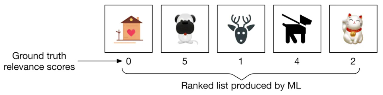
nDCG calculation process:

• Compute $\text{DCG} = { \sum_{i=1}^{p} {\text{relevance}_{i} \over {\log_{2}(i + 1)}}}$
  • $\text{DCG} = { {0 \over {\log_{2}(2)}} + {5 \over {\log_{2}(3)}} + {1 \over {\log_{2}(4)}} + {4 \over {\log_{2}(5)}} + {2 \over {\log_{2}(6)}} = 6.151}$
    • In this scenario, $p = 5$, but in practice $p$ will slide over a range of values and you chart them to see how well the system does in showing more and more recommendations
    • There's typically an "elbow" where after that, you have diminshing returns on showing new products
• Compute $\text{IDCG}_{p} = { \sum_{i=1}^{v} {\text{relevance}_{i} \over {\log_{2}(i + 1)}}}$
  • 
  • $\text{IDCG} = { {5 \over {\log_{2}(2)}} + {4 \over {\log_{2}(3)}} + {2 \over {\log_{2}(4)}} + {1 \over {\log_{2}(5)}} + {0 \over {\log_{2}(6)}} = 8.9543}$
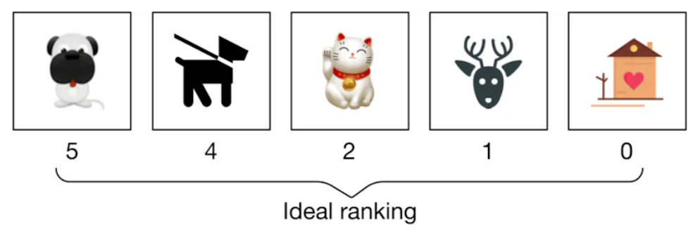
  • We see this is the "proper" ordering of the relevance list
• $\text{nDCG} = {\text{DCG} \over \text{IDCG}} = {{6.1} \over {8.9}} = 0.68$

Choosing Metrics

There are many choices that we saw above!

Precision, Recall, Precision@k, Recall@k, FCP, MRR, ARHR, MAP, MAP@k, or nDCG

They all have their pros and cons in terms of computation expense, ordering vs non-ordering (does position matter), binary vs continuous (relevant or not vs relevance score)

Some only make sense in the case of specific systems like RecSys, and others like nDCG wouldn't make sense in something like Entity Resolution out of the box - there's no "relevance score" on if 2 entities are the same, they either are or they aren't (I might get screamed at for this, but it's what I think)

Review:

• Precision and Recall
  • Precision@k measures the proportion of relevant items in the top $k$ results
  • Recall@k measures the proportion of relevant items retrieved in the top $k$ among the entire universe of relevant items
  • These are typically useful when you're interested in systems binary performance up to a specific $k$ cutoff point
    • They don't care about ordering, and they only focus on top $k$ so we may not get the full picture
• Fraction of Concordant Pairs (FCP)
  • Evaluates relative ordering of pairs
  • Useful in scenarios where relative ordering, without actual $i-j = \text{diff}$ is useful, is preferred and critical
  • It's actual comparisons end up exploding with $N^2$, but there are potential ways to avoid things like this, and obtaining this relevant ranking per user may prove difficult
• Mean Reciprocal Rank (MRR)
  • Based on ranking of first relevant item in the list
  • It's useful for focusing on that one specific item that is of the upmost importance
  • Can be useful when explicit relevance labels are missing and we have to rely on implicit signals such as a users choice among given list
  • Would be useful in things like Stack Overflow question answers or Search Engine results to see top ranked item
  • This metric fails to assess overall precision and accuracy of a recommended list
  • Best case scenario for when we want to quickly retrieve the top item, and maybe others, and ensure it's in our list (Candidate Generation?)
• Average Reciprocal Hit Rate (ARHR)
  • Extends MRR for all relevant items within the top $k$ positions
  • Averages out the reciprocal ranking, and so it does include relevance over the entire list
  • Useful in scenario's similar to MRR where we want to quickly retrieve top items, but the $1 - k$ all matter to us
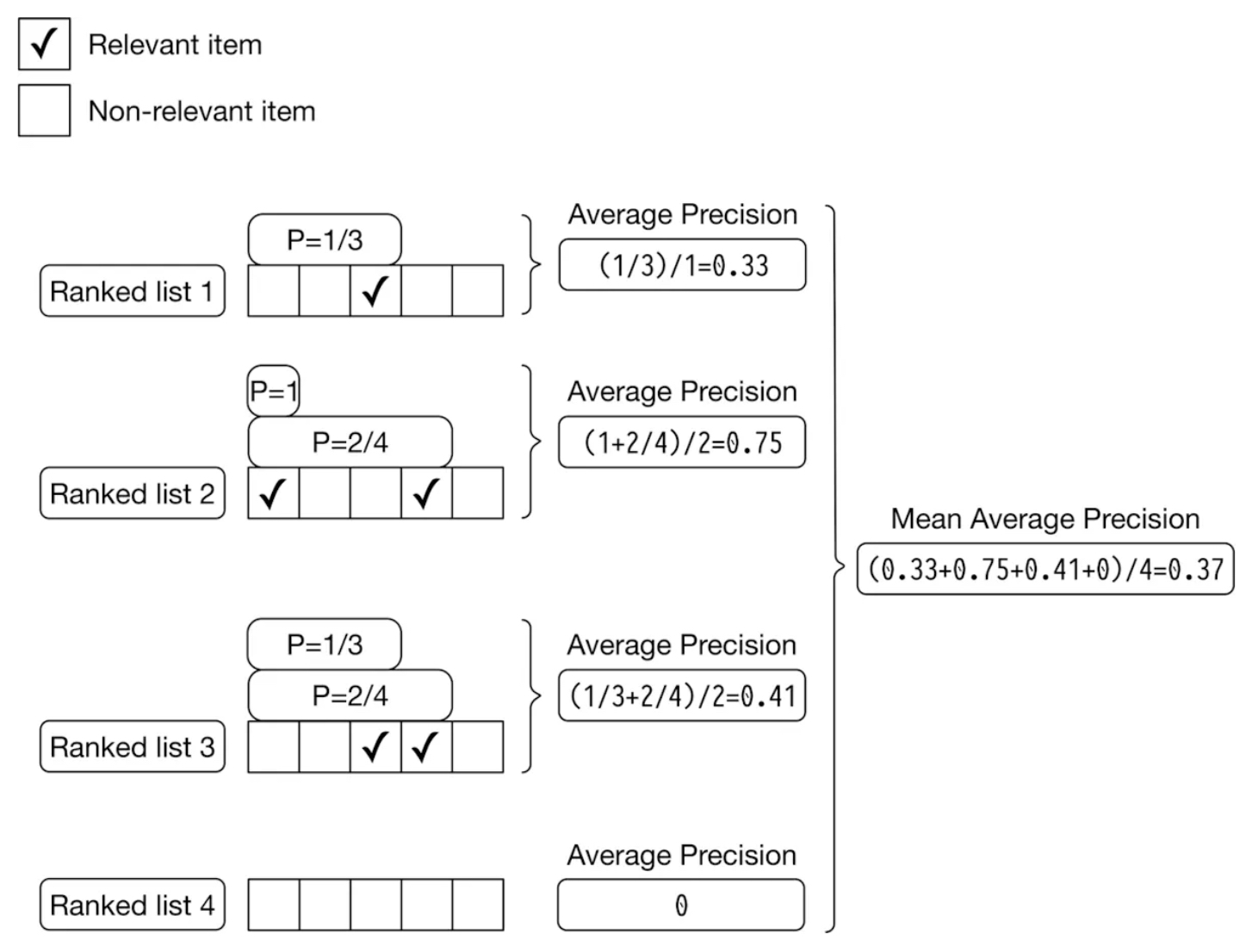
• Mean Average Precision (MAP)
  • Calculates average precision across multiple queries
  • Designed for binary relevance, and for taking into account the ranking of all relevant items
    • An event is either relevant or not
  • MAP evaluates how well all relevant items are ranked, rewarding systems that consistently rank relevant items higher
  • Not particularly useful when relevance is non-binary
• Normalized Discounted Cumulative Gain (nDCG)
  • Measures the quality of ranking by considering the position of each element in regards to the "ideal" recommendation list
  • Can handle continuous or binary relevancy scales
    • However, with binary scales it may be more appropriate to use MAP
  • Also handles relative positions inside of the list
  • Limitations are it's hard to find the actual "ideal" recommendation list, but in most ML Tasks there will be some form of similarity scores (embedding distance) between vectors, and we can use this to sort a list to find the "ideal" list

Train, Test, Validation Sets

A majority of the time the only way to get these metrics is by using source of truth sets - the most important being testing / validation sets

• Training Set: Used to actually train the model and update model weights
• Validation Set: Used throughout training or final model choice process, where we run a model over a holdout validation set to see enable us to choose the best model architecture
• Test Set: Running the final model over a dataset never seen before, and getting the final offline metrics

Validation Sets

In most supervised (or self-supervised) training scenarios you'll have validation holdout sets that can help you get these metrics, but for unsupervised learning or unseen supervised examples, you're a bit more stuck

Once you have your validation set, most of your offline metrics are easy to calculate!

A common example I've been apart of is Entity Resolution, where you may have some pairs deduped and matched in the past, but it represents a small subset of the total $TP$ true positives in your set

In these scenario's, you'll require human analysts or something like AWS Mechanical Turk to go through a larger selection of your universe to help you get to a validation set

Initially, bootstrapping a validation set might require $N^2$ total examples, but the main goal of having humans in the loop here is to reach $N \cdot K : K \lt N$ - basically we want to go from $\cdot N$ to $N \cdot K$

Example

Recommendation System examples

Candidate Generation

In Candidate Generation we select a set of items from a gigantic pool that would be relevant for a particular user - usually CG focuses on high recall, and wants to find any possible relevant links without missing anything

It tries to do this quickly, and typically won't use any large or complex models - overall it's goal is to reduce the search space while still keeping all true positives

In other systems like Search Engines, recall may not be the most important item to solve for at the end stages, because the denominator may be so humongous for some results that it completely bogs down the evaluation metrics - in these scenario's we'd want to focus on precision, ranking quality, or something else that accounts for the relevance / quality of ranking within those top-k items

Therefore, it's crucial to evaluate this because it's the foundation of our entire system! If it's too narrow or too broad you end up degrading the rest of the system as a whole

Ranking

Online Evaluation

Online evaluation revolves around live evaluation of a system running in production and serving users

Typically, a model is deployed and traffic is routed with some % split so we can perform A/B Testing on it - there's a system design case study around how this works. Users would be assigned to one of $A, B, ... , N$ services based on hashing of user_ID

The ultimate goal is to ensure the system works as intended in real world functions with respect to objective function and metrics

So as users are sent to different services we record information relating to business needs like Click Through Rate (CTR), Page Views, Site Time (how long they stay on website), Video View Time, etc...

A/B Testing can be used for any of the Stages listed above, and typically each one has separate metrics / business requirements

This all helps us to optimize hyperparameter configurations for params like regularization, learning rate, batch size, etc..While also allowing us to compare different functions for models like popularity based, personalized, diversity based, AND differnet objective functions like solving for optimal CTR, optimal time on site, or something different

Sometimes, solving for new video views will mean pushing click-bait to the top of the users feed, and this would come through during A/B Testing and feedback - at this point we may want to change the objective function we're solving for