CNN - Foundations, ResNet, DenseNet +

CNN Background

Images are just 2D arrays of numbers. Sometimes there are 3 separate 2D arrays, meaning an $N \times M \times C$ style matrix where there are $C$ channels of 2D matrices of size $N \times M$. The channels are usually Red, Green, Blue (RGB) for digital displays, and so with a $128 \times 128$ sized photo, if we have 100 of them, there will be an array of size $100 \times 3 \times 128 \times 128$

• 100 photos
• Each photo has 3 channels
• Each channel is a $128 \times 128$ grid

There are many many features of images, and the OpenCV toolkit helos with a lot of them - you can do a lot of analytics on images without any sort of ML or network.

• Checking lines is just finding a repeated array of black 0's surrounded by white 255's that are straight up and down
  • To do this the example above uses Gaussian Blur to soften each pixel based on it's surrounding values
  • Use Canny Edge Detection algorithm to find these areas
    • Gaussian Blue is needed as Canny is highly sensitive to noise
    • Canny uses gradients itself to find where a line is and where it's pointing
    • Some further post processing
    • Writing back lines in a distinct color onto the image
• Converting an image to greyscale
• Correcting skew
• etc

Anything you do with your hands on an iPhone can also be automated (and realistically is the same thing) as just doing it on OpenCV an iPhone typically shoots at 24 megapixels (MP) for a photograph, and a megapixel is exactly $1,000,000$ pixels. One million numbers for every single photo would be entered as a single example into a network, pipeline, etc. HD Resolution is defined as:

• $N$ rows is usually $1,280$
• $M$ cols is usually $720$
• That equates to $/approx 920,000$ pixels

So, there is a lot more input going into these pipelines compared to numeric, tabular data. How are these usually processed? By using pre-rolled transformations like stride, pooling, and other localized transformations to bring us from millions to thousands, along with other OpenCV like transformations to identify items inside of images versus just passing the entire thing in end-to-end

CNN's are convolutions of transformations passed over images, where there are layers of these transformations stacked on top of each other. In Where's Waldo, we can just scan each $T \times T$ section, and figure out if we can find Waldo's stripes based on line detections - this can be done because no matter where Waldo is, his features are the same

CNN's work well on image data - typical NN's will take an image, flatten it, and just pass it through a network. This is fine, but it doesn't generalize well across objects inside of images. Typical NN's aren't translationally invariant, but CNN's are!

There are some other principles - D2L AI talks about them below:

• In the earliest layers, our network should respond similarly to the same patch, regardless of where it appears in the image. This principle is called translation invariance (or translation equivariance)
• The earliest layers of the network should focus on local regions, without regard for the contents of the image in distant regions. This is the locality principle Eventually, these local representations can be aggregated to make predictions at the whole image level
• As we proceed, deeper layers should be able to capture longer-range features of the image, in a way similar to higher level vision in nature

From a high level, there are multiple layer types in CNN's:

• Convolutional layers take sliding windows (filters / kernels) over pixels to extract local features like edges and textures. Each filter produces a feature map by aggregating pixels in it's window
  • Convolutions also add $b$ bias weights to the output scalar
• Pooling layers will reduce the actual spatial size of feature maps by sliding a window and applying an aggregate function (max, avg, etc) to that region
• Dense layers (fully connected layers) have each neuron connected to another next layers neurons, and these are for combining features from above layers
• Activation layers look to take these other layers and look for features by utilizing non-linear functions such as ReLU, sigmoid, tanh, etc to introduce non-linearity inside of the network

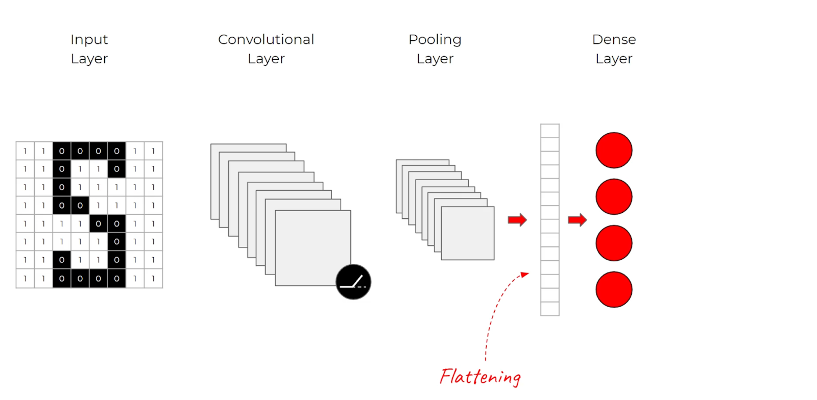
Instead of flattening inputs, CNN's apply filters by utilizing convolutional and pooling layers. These filters stride over the entire input image or hidden layers

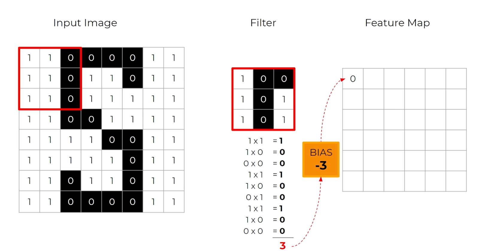
ReLU layers also allow CNN's to find edges, textures, etc because color gradients will change from -1 to 0 and other features, and pooling layers inbetween help reduce the size of the problem space as it grows. All of this ends up being passed into final softmax layers and other things to predict image classes, output bounding boxes, etc.

Translational Invariance

Translational invariance is the property of a system that remains unchanged when its position or input data is shifted in space. It's important because generally we're more interested in the presence of a feature versus where it's actually at - once a CNN is trained to detect things in an image, changing the position of that thing in an image won't prevent the CNN's ability to detect it

If we utilized every pixel in a single megapixel image to map to a hidden layer, we would beed $10^12$ parameters. Each megapixel image contains $1000 \times 1000$ pixels, and so mapping each of these into a single hidden layer of the same size would be $1000 \times 1000 \times 1000 \times 1000$ - completely infeasible, and also hard for the model to discern a pixel above and below another pixel are related to it!

Translational Invariance above helps fix that a bit, as it implies a shift in the input $\bold{X}$ shoudl simply lead to a shift in the hidden state $\bold{H}$, and that shift shouldn't depend at all on the pixel location. That leads to the below mapping across an input $\bold{X}$

$\bold{H}_{i,j} = u + \sum_{a} \sum_{b} \bold{V}_{a,b} \bold{X}_{{i+a}, {j+b}}$

The above equation just means, for each of the column indexes $j$, we setup some sort of box of size $b$. That would give the horizontal pass across columns, and we'd do that for each row $i$, and pass over a number of rows $a$ from $i$ - it's just a box! Add the final bias term $u$ to the final output of that sum, and that's the value for the hidden state at location $\bold{H}_{i,j}$

The above is the definition of a convolution

Locality

Translational Invariance and convolutions above showcase some of the ways that locality is present in these models. Each pixel is sent to the hidden state based on surrounding, localized, pixels. The same subset in the different places in the input should produce the same results, and the subset is defined by its local region

Therefore, translational invariance and locality are two peas in the same pod. However, the locality principle is more focused on the fact that the size of $a, b$ above in that formula should never have to be very large in order to glean relevant information for $\bold{H}_{i, j}$. There should be some magic range $a, b > \Delta$ such that $\bold{V}_{a,b} = 0$, which means we shouldn't look outside of some localized range around $i, j$. Formally, we can just use the matrix $\bold{V}$ as a set of learnable parameters to do this

$\bold{H}_{i,j} = u + \sum^{\Delta}_{a=-\Delta} \sum^{\Delta}_{b=-\Delta} \bold{V}_{a,b} \bold{X}_{{i+a}, {j+b}}$

The above equation is a convolutional layer and $\bold{V}$ is the convolutional kernel / filter

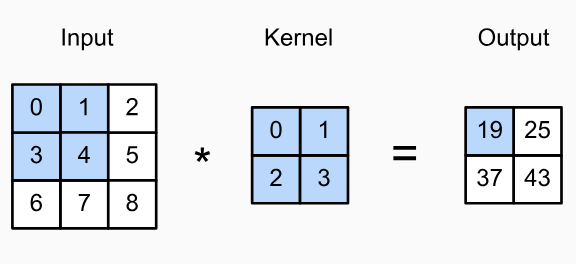
The above requires much less computation power compared to the fully mapped hidden layer described at the top. More on the order of hundreds compared to millions

Convolutions

The last principle states that deeper layers should represent larger and more complex aspects of images, which can be achieved by interleaving nonlinearities and convolutional layers repeatedly

i.e. we can use a bunch of convolutional layers + non-linear functions stacked as components to create representations of things like circles, boxes, cats, dogs, etc

The convoluations in math section below goes into what convolutions measure, but the functions end up being very similar over 2D tensors. Convolutional layers actually use cross correlation to find the overlap of two functions

$(f \ast g)(i,j) = \sum_{a} \sum_{b} f(a,b)g(i + a,j + b)$

There are some cosmetic signage changes between + and -, but ultiamtely we're just checking over a box how strongly $f$ and $g$ relate to eachother. The above convolutional kernel / filter, is how we will traverse images and detect shapes

Convolutions In Math

In math, a convolution is a way of blending two functions together to see how one shapes the other over time - at any given moment it helps to calculate the overlapping area of one function while a second function is flipped, slid across the first, and multiplied point by point

We want to know for a specific stimulus at time $\tau$, what the response is at some time $t$

The reason for flipping, sliding, and multiplying:

• Flipping the function $g(\tau)$ to $g(-\tau)$ creates a mirror image across the vertical axis
  • In signal processing the oldest (first) signal corresponds to the systems first response
  • You don't actually "flip" the function physically, you just query it at $t - \tau$
• Sliding $g(t - \tau)$ shifts the functions along the horizontal axis by a variable time delay, and this usually corresponds with furthering the response as well by time $t$ to keep the functions in sync
• Multiplying the two together just gives the overlap
  • $f(t) \times g(t - \tau)$

The flipping part is the most confusing to me, but the general idea is that if there's a signal at time $\tau$, we can measure the total response at time $t$, and so the time pass between stimulus and response is $t - \tau$

If we slid $g$ across $f$ without the flip, we'd just have $\int f(\tau)g(\tau + t)d_{\tau}$ which is cross correlation. CNN's do implement cross correlation, which is similar to an inverse of convolutions.

$(f \ast g)(t) = \int f(\tau)g(t - \tau)d_{\tau} \rarr g(t-\tau) = g(-(\tau - t))$

The response function $g$ requires the elapsed time to have occurred, and so the system response according to $g(t - \tau)$. Therefore, flipping $g$ and comparing it to $f$ allows us to compare the response effect after $t$ delay to each signal. If a stimulus occurred at $\tau = 3, 12, 18$, their corresponding ages at $t = 20$ would come out to $20 - [3, 12, 18] = [17, 8, 2]$ so evaluating $g(17), g(8), g(2)$

• $g(17)$ here relates to "how much response does a single impulse produce 17 time units after it occurred"
• By multiplying $g(17)$ by the function $f(20)$, we get to see how a response at time $t=20$ is effected by a signal at time $3
• $f(t)$ = amount of drug injected at time $t$
• $g(\tau)$ = concentration in the bloodstream $\tau$ hours after one injection
  • To check the concentration at $t=20$, the injection is now 17 units old, so the contribution from that injection is $f(3) \cdot g(17)$

Altogether, we are checking response at time $t$: $t = \sum_{\tau} \text{stimulus f}(\tau) \times \text{response after g}(t - \tau)$

Channels

There are usually 3 channels in images - Red, Blue, Green (RGB), and so each filter box is actually $H \times W \times C$ as a 3-D tensor instead of a 2-D box. This box can be indexed as $\bold{[X]}_{i,j,k}$

Mapping these to single value hidden layers usually reduces expressiveness, and so in most cases each channel (RGB) is mapped to it's own hidden state tensor as well

$\bold{[H]}_{i,j,d} = \sum_{a=-\Delta}^{\Delta} \sum_{b=-\Delta}^{\Delta} \sum_{c} \bold{[V]}_{a,b,c,d}\bold{[X]}_{i+a,j+b,c}$

Which is a disgusting formula to read:

• $i, j$ are the pixel locations, and $a, b$ are the offsets of the convolutional kernel / filter
• $c$ is the input channel
• $d$ is the output channel

So ultimately the interpretation is run a bounding box around pixels $i, j$ of size $a, b$ for all channels $c$ and map the filter to a hidden state at location $i, j$ with $d$ channels

For example, suppose:

• Input image is $224 \times 224 \times 3$
  • Therefore, $c = 3$
• Kernel size is $3 \times 3$
  • Therefore, $a = b = 3$
• We desire $64$ output channels
  • Therefore, $d = 64$
  • In this case, there would be 64 different filters! Each of these $d$ filters are $a \times b \times c$
• One singular value $H_{i,j,d}$ represents the feature map $d$ at location $i, j$
  • $i = 40$
  • $j = 90$
  • $d = 17$
  • "What is feature map #17 at pixel (40, 90)"
  • To compute this take the $3 \times 3 \times 3$ patch centered at (40, 90), run filter $V_{d}$ #17 over it, multiply every element, sum it together
  • This produces one single scalar $H_{40, 90, 17}$

At the end

$$H_{i,j,:} = \begin{bmatrix} H_{i,j,1} \\ H_{i,j,2} \\ ... \\ H_{i,j,64} \end{bmatrix}$$

An easier way to view this all is: $\bold{[H]}_{i,j,out} = \sum_{a=-\Delta}^{\Delta} \sum_{b=-\Delta}^{\Delta} \sum_{c} \bold{[V]}_{a,b,in,out}\bold{[X]}_{i+a,j+b,in}$

Why use channels? They mostly allow a more complete set of complexity to be represented that may be lost due to restricting the CNN to local filters over images. There may be thousands of input channels besides just RGB as well, and sometimes we need a different mapping between in and out channels. The usage of thousands of filters is evident in the line detection kernel example where one single kernel allows us to find exactly up and down vertical lines, but we may need thousands of channels to get features like "slight curve" or "elbow edge", etc

Multiple Input and Output Channels

When there are multiple input channels, the general idea is to perform the cross-correlation operation over each channel, and somehow aggregate the results at the end. Most often this is a sum of the cross-correlation output, but it could be anything like average, max, min, or even multiplying each by yet another filter!

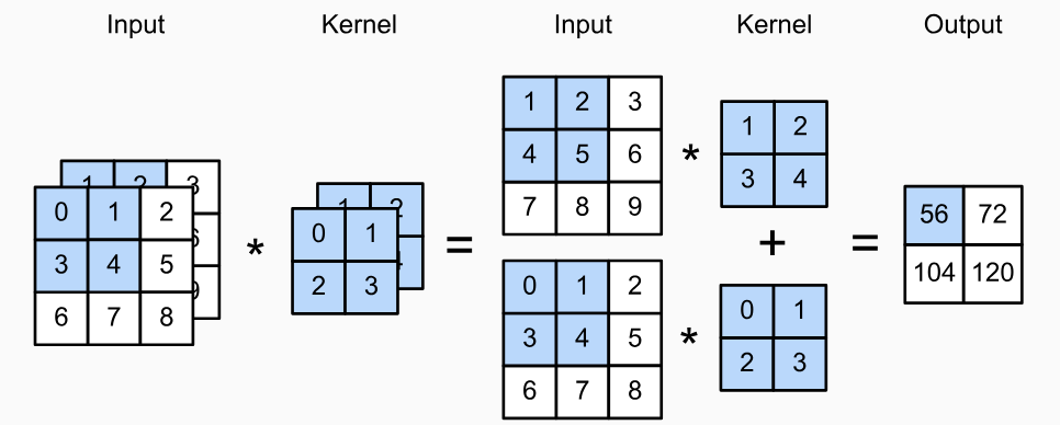
Utilizing multiple channels in each output layer is also useful. In most CNNs, the number of channel dimensions actually increases as the network goes on, as you downsample the total size of the image and create more features at that exact spot. Intuitively if you're looking at a $1,024 \times 1,024$ image, you don't really need the million pixels in a grid. At each sub-image we pass over with our cross-correlation box, there may be features we look to extract from that specific spot. If we have potentially thousands of features we want to check at each spot, this usually is easiest done as thousands of channels - each filter / channel can look for different lines, patterns, circles, etc. The total number of channels is known as channel depth, and it usually increases further down the network as total image size decreases

Each channel is not really a feature in it of itself, but when you combine thousands of them, downstream channels can become quite expressive by finding circles, stars, and other patterns frmo combinations of less expressive channels upstream

To find the dimensions of all this it would be:

• $c_i$ is the number of input channels
• $c_o$ is the number of output channels
• $k_h \times k_w$ is the kernel size
• We would have a kernel of size $c_i \times k_h \times k_w$ for each output channel - meaning if we have 10 output channels and 3 input channels, we would need to produce 10 kernels in total, and pass each of them over the input
  • If we have one output channel, a kernel of size $c_i \times k_h \times k_w$ makes sense
  • If we needed two, we'd need another
  • ...
• Concatenating each of the $c_i \times k_h \times k_w$ kernel outputs as the final output gives the desired final $c_o$ output channel tensor

Given an image of size $h \times w$, the cost for computing a $k \times k$ convolution is $O(h \cdot w \cdot k^2)$, and if we increase the input and output channels beyond one it becomes $O(h \cdot w \cdot k^2 \cdot c_i \cdot c_o)$ as we need to:

• Traverse the entire $h \times w$ image for every kernel ($h \times w$)
  • Multiply the kernel by the image ($k^2$)
    • Then do that for every channel ($c_i \times c_o$)

Which is quite expensive. For a $256 \times 256$ pixel image with $5 \times 5$ kernel and $128$ input and output channels, it comes to 53 billion operations

Feature Examples

Using the above basic layers, there's a lot than can be done

There are lots of packages that run this, and there are even ways to distribute this. If you have a $1,000 \times 1,000$ image, you could send rows $[0, 502]$ and rows $[498, 1,000]$ to 2 separate nodes, and each of them can map their result sets to a hidden layer computed on node 3 - this is known as spatial parallelism or halo exchange

There's much more about this in Training, Hardware, and Parallelism

Line Detection Kernel Example

The general idea is if we have perfectly up and down lines, we can use a kernel of $[1, -1]$ as our filter. If two horizontal cells are the same, they'll output 0, if they're different this will result in a non-zero difference

If our photo is just of a single grey-scale channel of all white 255's and all black 0's, then this produces a valid vertical line detection kernel. It's a nice and cool thing if we know exactly how to express the kernel filter, but rarely can we formalize every single kernel in existence

The general idea about learning kernel's is described below - the general idea is we have an input $X$ and an output $Y$ where $Y$ was somehow created from $X$ - it's not a direct up and down line, it's just something that a black box created. How can we learn the transformation that created $Y$ from $X$?

If you know both $Y$ and $X$ you can uncover the convolutional kernel using gradient descent. It will continuously tweak the kernel conv2d so that the loss is continuously minimized

Show Python Script

# Construct a two-dimensional convolutional layer with 1 output channel and a
# kernel of shape (1, 2). For the sake of simplicity, we ignore the bias here
conv2d = tf.keras.layers.Conv2D(1, (1, 2), use_bias=False)

# The two-dimensional convolutional layer uses four-dimensional input and
# output in the format of (example, height, width, channel), where the batch
# size (number of examples in the batch) and the number of channels are both 1
X = tf.reshape(X, (1, 6, 8, 1))
Y = tf.reshape(Y, (1, 6, 7, 1))
lr = 3e-2  # Learning rate

Y_hat = conv2d(X)
for i in range(10):
    with tf.GradientTape(watch_accessed_variables=False) as g:
        g.watch(conv2d.weights[0])
        Y_hat = conv2d(X)
        l = (abs(Y_hat - Y)) ** 2
        # Update the kernel
        update = tf.multiply(lr, g.gradient(l, conv2d.weights[0]))
        weights = conv2d.get_weights()
        weights[0] = conv2d.weights[0] - update
        conv2d.set_weights(weights)
        if (i + 1) % 2 == 0:
            print(f'epoch {i + 1}, loss {tf.reduce_sum(l):.3f}')

Feature Map

Convolutional layer outputs can also be called feature maps, since they can be treated as learned representations, or features, in the spatial dimensions to the subsequent layer. I.e. they can be considered learned representations from their input layer that they extend to their output layer

The receptive field of any element $x$ in some random layer is the collection of all elements in the previous layer that may affect the calculation of $x$ during the forward propogation. This is similar to understanding the partial derivative as items move through the chain of calculations - if there's a partial derivative $\gt 0$ then the receptive field of a layer would include that field

Padding and Stride

If our image is of size $n_h \ times n_w$ and the convolution kernel shape is $k_h \ times k_w$, then the output shape would be $(n_h - k_h + 1) \ times (n_w - k_w + 1)$

Padding and striding are ways to either reduce, increase, or alter this final output size. Maybe we want more, less, or just different final output shapes than the ones above

Padding

The below is a pixel utilization chart which shows how much any pixel is used with a kernel of size $n \times n$

The corner pixels are essentially always have a utilization of 1 - to solve this, we can pad the images so that all of the pixels are in the "central" part

Because of this, CNNs commonly use convolution kernels with odd height and width values which allows preserving dimensionality while padding the same amount on top and bottom. If we pad the top, bottom, and each side with 2 then we're able to use a convolution of size 3 without any weird edge cases

Stride

During our cross-correlation computations above, we slide one by one over each window in our summation - strides would be increasing that size from 1 to some other number

Striding ultimately reduces the output size by a multiple of the stride size - going from 1 to 2 ultimately halves the total output size

Pooling Layers

Given we can have thousands of channels spread over tens to hundreds of layers, how do we actually get some global aggregate information over the entire image?

Pooling layers help to aggregate, or pool, information across channels, pixels, layers, etc into global information stores. By gradually aggregating information, yielding coarser maps, and building larger overall features, we accomplish the goal of learning global representations and features. The deeper into a network, the larger the potential receptive field (relative to the immediate input layer) that each hidden node is sensitive to

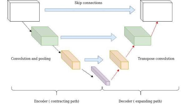
Foreshadowing - sometimes we want global information while also keeping channel based features. This is where skipnets and resnets come in. They allow keeping global informative features within a layer without losing the granularity of channels. Combining them loses some information, but ultimately both can be used in parallel with skip levels

Pooling layers are similar to cross-correlation functions in that they are fixed size windows (pooling windows) traversing over layers, except the output is mostly around aggregating to a singular value. There is no filter / kernel - there's simply no need for it!

Most pooling layers are maximums, sums, or averages. Pooling is effectively downsampling an image - you take 4, 9, 16, etc pixels and essentially aggregate them into a global pixel representing all of them

Padding and Stride are also used for these layers, and are the exact same as cross-correlation. That being said, since pooling layers aggregate information from an area, typically the stride is the same size as the kernel dimension

Multiple input channels are also handled in aggregate where pooling is just done over each input channel to produce an effective output channel. It doesn't make much sense to alter input different than output unless you use different pooling types. If you want to use both max and average pooling, you'd just be making $c_o = 2 \cdot c_i$

LeNet

The first digital ImageNet number detection CNN was created by Yann Lecun - it consists of:

• A convolutional encoder consisting of two convolutional layers
• A dense block consisting of three fully connected layers
• There are 10 outputs in the final fully connected layer, which could be swapped with a softmax activation function to describe the probability of being any digit 0-9

There's a great website / article by sbondaryev on this with much better images / playground

The input image would be $28 \times 28$, it would get sent through 4 layers of convolutions and average pooling, followed by 3 layers of fully connected

LeNet also utilizes sigmoid activation funcations at the end of each 2D Convolution - this sigmoid is applied to every pixel coming out of the 2D convolutio itself. These are called squashing activations inside of the network. Digits are recognized by how its features relate to eachother, not by their pixel positions in the image itself - the number could be in part of the image itself; It's local and translationally invariant!

The output layer itself is not a softmax classification of the 10 possible digits, it's something very different. Each of the 10 potential outputs holds a fixed $7 \times 12$ pattern, there's one pattern per class. The layer before the last is of size $(1, 84)$, which is $7 \times 12 = 84$. That second to final dense layer were chosen to match these patterns, and essentially allow mapping the output of any image onto the same $7 \times 12$ grid. The final *radial basis function (RBF) computes the difference between each potential digit and the one passed through the network - whatever one has the smallest distance is the chosen class.

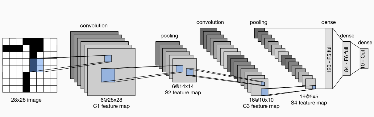
The below python produces the following output:

Conv2D               (1, 28, 28, 6)
AveragePooling2D     (1, 14, 14, 6)
Conv2D               (1, 10, 10, 16)
AveragePooling2D     (1, 5, 5, 16)
Flatten              (1, 400)
Dense                (1, 120)
Dense                (1, 84)
Dense                (1, 10)

Epoch 1/10
469/469 ━━━━━━━━━━━━━━━━━━━━ 10s 21ms/step - accuracy: 0.1018 - loss: 2.3085 - val_accuracy: 0.1000 - val_loss: 2.3085
Epoch 2/10
469/469 ━━━━━━━━━━━━━━━━━━━━ 11s 24ms/step - accuracy: 0.1059 - loss: 2.3041 - val_accuracy: 0.1000 - val_loss: 2.2969
Epoch 3/10
469/469 ━━━━━━━━━━━━━━━━━━━━ 11s 22ms/step - accuracy: 0.2186 - loss: 2.1957 - val_accuracy: 0.4717 - val_loss: 1.7799
Epoch 4/10
469/469 ━━━━━━━━━━━━━━━━━━━━ 10s 21ms/step - accuracy: 0.5319 - loss: 1.3382 - val_accuracy: 0.5858 - val_loss: 1.1263
Epoch 5/10
469/469 ━━━━━━━━━━━━━━━━━━━━ 12s 26ms/step - accuracy: 0.6057 - loss: 1.0367 - val_accuracy: 0.6458 - val_loss: 0.9725
Epoch 6/10
469/469 ━━━━━━━━━━━━━━━━━━━━ 11s 23ms/step - accuracy: 0.6565 - loss: 0.9127 - val_accuracy: 0.6679 - val_loss: 0.8768
Epoch 7/10
469/469 ━━━━━━━━━━━━━━━━━━━━ 9s 19ms/step - accuracy: 0.6882 - loss: 0.8395 - val_accuracy: 0.6914 - val_loss: 0.8234
Epoch 8/10
469/469 ━━━━━━━━━━━━━━━━━━━━ 10s 21ms/step - accuracy: 0.7064 - loss: 0.7883 - val_accuracy: 0.7072 - val_loss: 0.7793
Epoch 9/10
469/469 ━━━━━━━━━━━━━━━━━━━━ 9s 19ms/step - accuracy: 0.7207 - loss: 0.7418 - val_accuracy: 0.7210 - val_loss: 0.7390
Epoch 10/10
469/469 ━━━━━━━━━━━━━━━━━━━━ 9s 20ms/step - accuracy: 0.7342 - loss: 0.7011 - val_accuracy: 0.7391 - val_loss: 0.6995

Show Python Script

import tensorflow as tf

class LeNet(tf.keras.Model):
    def __init__(self, num_classes=10):
        super().__init__()
        self.net = tf.keras.Sequential([
            tf.keras.layers.Conv2D(
                filters=6,
                kernel_size=5,
                padding="same",
                activation="sigmoid"
            ),
            tf.keras.layers.AveragePooling2D(
                pool_size=2,
                strides=2
            ),
            tf.keras.layers.Conv2D(
                filters=16,
                kernel_size=5,
                activation="sigmoid"
            ),
            tf.keras.layers.AveragePooling2D(
                pool_size=2,
                strides=2
            ),
            tf.keras.layers.Flatten(),
            tf.keras.layers.Dense(120, activation="sigmoid"),
            tf.keras.layers.Dense(84, activation="sigmoid"),
            tf.keras.layers.Dense(num_classes)
        ])
    def call(self, x):
        return self.net(x)

model = LeNet()

x = tf.random.normal((1, 28, 28, 1))

for layer in model.net.layers:
    x = layer(x)
    print(f"{layer.__class__.__name__:20} {x.shape}")

(x_train, y_train), (x_test, y_test) = \
    tf.keras.datasets.fashion_mnist.load_data()

x_train = x_train.astype("float32") / 255
x_test = x_test.astype("float32") / 255

x_train = x_train[..., None]
x_test = x_test[..., None]

batch_size = 128

train_ds = (
    tf.data.Dataset
        .from_tensor_slices((x_train, y_train))
        .shuffle(10000)
        .batch(batch_size)
)

test_ds = (
    tf.data.Dataset
        .from_tensor_slices((x_test, y_test))
        .batch(batch_size)
)

model.compile(
    optimizer=tf.keras.optimizers.SGD(learning_rate=0.1),
    loss=tf.keras.losses.SparseCategoricalCrossentropy(
        from_logits=True
    ),
    metrics=["accuracy"]
)

model.fit(
    train_ds,
    epochs=10,
    validation_data=test_ds
)

Continuing CNNs

After LeNet was released, there was a general "winter" of CNN exploration, usage, and continuation. There were lots of reasons for this, most I don't know, but the most interesting pieces were the feature engineering, data, and hardware at the time.

Most pipelines at that time were doing feature engineering before feeding inputs into the CNN:

• Image centering
• Greyscale processing
• Reconstruction, splitting, etc

These features were being processed before anything went into a model, and running these feature pipelines was expensive. In 1999 NVIDIA GeForce 256 could process $480,000,000$ (480 MFLOPS) per second, whereas today can perform $\gt 1,000,000,000,000,000$ (1000 TFLOPS, or 1 PFLOP) per device

So back then you had to find a number of expensive images stored digitally, process them with analytical tools, open source software, and image processing toolkits, feed that through a standard feature extractor for images, and finally place this into a classifier. This was extremely expensive for the hardware at the time!

After that, AlexNet was able to show that lower layers of CNNs can learn the features, given enough compute power and data. These lower layer features are able to be extended to higher level layers for more prominent features like noses, circles, dogs, etc.

Separately, the use of GPU's over CPU's allowed for significant matrix computations to be done on the order of TFLOPS per second, which is extremely necessary for convolutional networks which are doing thousands of matrix computations. The significance of quantization cannot be overstated - for 16 bit floating point it's on the order of 300 million BFLOAT16 operations per second compared to 20 million FP32 for general 32-bit floating point numbers. CPU's rarely get over 1 TFLOPs, but they handle a large range of other logic besides matrix-matrix calculations

AlexNet

AlexNet won the ImageNet Large Scale Visual Recognition Challenge in 2012, and was the first model to show that learned features can outperform manually designed features.

AlexNet is not very different from LeNet, it's mostly just an extended model with more layers which allowed for more features. Adding more convolutional layers with more channels required more compute and more data. With that, it won the competition!

There are many other small tweaks in the name of training optimizations like using ReLU instead of Sigmoid

Training - Batch Normalization

Training these CNNs is damn near impossible. Convergence never seems to come, there's memory issues, a loss of seeing an increase in loss, and many other typical pitfalls from ML. They are even more apparent when working with pixels in a small range of $[0, 255]$ that go through thousands of even more filtering and reduction operations, sooner or later it's just minimal updates in any direction.

ReLU helps with this and avoiding vanishing gradients, other tweaks with activations can help too, but none help as much as batch normalization. Batch normalization consistently helps with convergence, and can help alleviate a lot of these small issues with some light batch processing techniques

The intuition behind this comes from standardizing vectors as input to MLP's and other linear models. The entire reason we standardize to mean = 0 and variance = 1 is because it ensures model variables all sit on the same playing field, and ensures they don't become to unwieldy. It also helps on explaining what's going on inside the models, but ultimately it just helps on passing the data through the model. If your input can become arbitrarily large, a model can implement much more violent decision boundaries. If the inputs are constrained to a smaller range, the model is forced to learn smoother, simpler functions. The main idea is we want to reduce the volatility to weight updates as our network produces - even if it takes a bit of time for it to converge, the convergence is smoother versus large, bouncing, violent updates

If $z = w^{T}x$, and $x = [1000, 500, -700]$, then a tiny change to $w$ can produce an enormous change in $z$ given the $x$ values are so large. Simply because $x$ is large doesn't mean we want to make large updates to our weights

If we normalize it to $x = [0.4, -0.2, 1.1]$, the same change or loss would produce a much smaller update, and ultimately reduces steep response updates

The idea of batch norm is to normalize the batch itself to have mean of 0 and unit variance over a mini batch. The inventors of batch normalization postulated that this drift in the distribution of variables, whether in the input or along the multiple layers of the network, could hamper the convergence of the network. If one layer has activations 100 times larger of any other layer, maybe due to some odd activation function, this might necessitate compensatory adjustments to the learning rate - there's no reason the updates from that layer shoud contribute 100 times as other layers

Batch normalization is applied to individual layers at a time. In each training iteration we normalize the inputs by subtracting their mean and dividing by the standard deviation, calculating these off of the mini batch itself. Lastly a scale coefficient and offset is applied to recover some lost degrees of freedom

If $\Beta$ is a minibatch, and some $x \in \Beta$is an input to Batch Normalization $BN(x)$, it would be defined as

$BN(x) = \gamma \cdot {{x - \hat{u}_{\Beta}} \over \hat{\sigma}_{\Beta}} + D$

As a result, this minibatch would have zero mean and unit variance. The $\gamma$ and $D$ variables are 2 new variables introduced that must be learned, which brings the degrees of freedom back up 2.

In fully connected layers, batch normalization is done before activation functions: $h = \phi (BN(\bold{Wx + b}))$

In convolutional layers, batch normalization happens after the convolution but before the non-linear activation function. Batch normalization happens on a per channel basis across all locations

Once this model is learned and trained, batch normalization is calculated over the entire input dataset.

ResNets

Learning better networks isn't as easy as just simply stacking more and more of those above layers on! Unlike NLP, where more attention layers allow for better embedding representations, CNN's showed diminishing returns and sometimes complete degredation when stacking more of these layers together. They also had problems with vanishing and exploding gradients from the millions of numeric multiplications across small floating point numbers. Vanishing gradients are related to degredation, but they are technically distinct problems that could be solved with separate architectures like batch normalization. Furthermore, CNN's mostly create new features by utilizing convolutional layers + pooling, but the more pooling we do the more channel features we sum up and fail to preserve upstream information. The more hidden layers, the more the information from the original input gets lost. ResNets attempt to solve this by allowing those convolutional channel features to continuously be reused with skip / residual connections, batch normalization across hidden layers, and by doing some fancy tricks with residual connections.

Vanishing gradients are commonly talked about with ResNets as well, and while they weren't the intended focus of the original paper, they did help further the solution. When using batch normalization on even deeper layers, researchers did see networks converge (no more vanishing gradients), however the accuracy results were still degrading. So ultimately mixing batch normaliztaion and skip / residual connections together allowed for deeper networks that converged without degredation!

To be clear, the initial ResNet paper strictly sought out to solve How to create deeper models so that they perform definitely better than shallower models - this is discussed in the resnet function class math section. That being said ResNets helped with the latter two problems of gradient issues and information preservation

The architecture of ResNet comes down to utilizing skip / residual connections $I(x)$ instead of just using some activation $F(x)$ - $y = F(x, W_i) + I(x)$

In doing so, we ensure upstream layers are able to be reused, and furthermore if the $F(x)$ function does nothing useful (degrades), we can just learn to set it to 0. The core of the paper is that learning $F(x) = 0$ is much easier than learning $F(x) = I(x)$ - that's it! In doing so we help to solve the 3 major problems of degredation, vanishing gradients, and information loss; The extra trick of batch normalization also helps vanishing / exploding gradients together

The use of residual connections to solve the deeper model = degredation problem helped to also solve some extra side problems. This was showcased by the ResNet-18's ability to outperform other models and win 2015 Large Scale Visual Recognition Challenge

ResNet Function Class Math

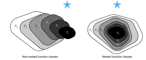
The general thought behind ResNets, and ultimately the whole "bigger is better" model continuation, deals with function class families. If we have some function family $\bold{F}$, which represents the class of functions a specific network architecture can reach, then for all $f \in \bold{F}$ there exist some set of weights and biases that obtain $f$ through training on a suitable dataset. If there is some magical $f^{*}$ that describes our black box we need to find, we mostly just care if $f^{*} \in \bold{F}$. We may approximate $f^{*}$ with the best function $f^{*}_{\bold{F}} \in \bold{F}$ as our best function inside of $\bold{F}$ that is close to the magic one

Again, to be clear, the initial ResNet paper strictly sought out to solve How to create deeper models so that they perform definitely better than shallower models. If the shallower model was the better choice, then the last layer of the model isn't needed and we can set $F(x) = 0$ in this case, which is much easier than getting it trained to $F(x) = I(x)$. Without the skip / residual connections, this mapping is much harder to learn

Regularization can control the complexity of $\bold{F}$ and achieve consistency, which means a larger set of training data can lead to better and better $f^{*}_{\bold{F}}$

If we propose a new bigger and better architecture $\bold{F}^{'}$, we should hypothetically have a larger set of functions to choose from, and we'll either get a better $f^{*} \in \bold{F}^{'}$ or the same one as before from $\bold{F}$. This is only true if $\bold{F} \subseteq \bold{F}^{'}$

If the above is not true, then something like $\bold{F}^{6}$ below may be worse off, even though it's larger, than $\bold{F}^{3}$

ResNet Function Example

If we have a 10 layer network $\bold{F}_{10}$ and we insert another $\bold{F}_{11}$ via a fucntion $g(x)$, we'd be effectively turning it into $f(x) = g(x) + x$. This isn't completely true, but it's close enough

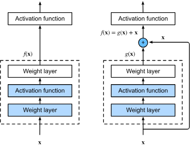
If we didn't add $+ x$ at the end, then to recover the original function and ensure that $\bold{F}_{10} \subseteq \bold{F}_{11}$, we would need $g(x) \rarr x$. That being said, for any layer, getting $\sigma(Wx + b) \rarr x$ is quite difficult. ReLU isn't an identity function for negative inputs, sigmoid is almost never an identity, and linear layers require $W = I, b = 0$ which may never be the case during training. Although $\bold{F}_{11}$ contains $\bold{F}_{10}$ mathematically, it may never actually find it, however we can be sure that $\bold{F}_{10}$ is a proper subset. So how did the authors propose to solve this? Just add in $+ x$ at the end! Forcing $g(x) \rarr 0$ is much easier

The degredation problem stated out is when $\bold{F}_{11}$ is actually worse than $\bold{F}_{10}$, which means the new $g(x)$ included layer is struggling to find the identity function, and the new layers we have are even worse than just having stayed with $\bold{F}_{10}$, because we never added $x$ at the end and it couldn't converge to $I(x)$

ResNets help the degredation problem by bringing $x$ along additively instead of forcing $g(x)$ to learn the identity function. In doing so, if the extra layer is struggling to find any better function fit, it can tend towards $g(x) \rarr 0$, which is infinitely easier to learn. In the examples above, if $f(x) = g(x) + x$, the network can learn $g(x) = 0$ and we just continue on with $\bold{F}_{10}$. Pushing $g(x)$ to 0 is much easier than forcing $g(x) = I(x)$ as well

ResNet Theory / Background

The general theory was then for deep neural networks, if we can take any architecture and stack on some new layers that learn $f(x) = g(x) + x$, then the new architecture would be a strict superset of the old one. It for sure contains the old one, and it may contain new areas of exploration

Residual Learning is useful because it allows very deep networks to be trained by reformulating the layers as learning residual functions with reference to the layer inputs, rather than directly learning unreferenced functions. This helps address vanishing gradient problems, and also enables effective training of much deeper architectures

There was a huge issue of exploding / vanishing gradients, along with overall degredation of accuracy in these models, that were solved by utilizing normalization layers and residuals - ResNets usage of residual skip conncetions specifically addresses the degredation problems.

Why? The general idea is if $f(x)$ is the desired underlying mapping we want to learn for the activation function at this layer, then in the "old" way we directly have to learn $f(x)$ entirely. With a residual block, $g(x)$ only has to learn $f(x) - x$

Small Aside On Intent Of Paper

Again - why is that useful? If there's no better expressive model we find with $g(x)$, and the best course of action is to continue with $x$, we can just set $g(x) = 0$. This is a specific implementation of a multi-branch block, where one of the two branches is the identity function

Again, again, again - why does this help us learn $f(x)$ which was the original goal? This is not the intuition - the main intuition is that If the optimal function happens to be close to the identity in some layer, then learning the difference (i.e. $g(x) = 0$) is much easier than learning the identity function from scratch. Learning the identity function is extremely difficult! That's the entire intuition - learning the difference is easier than learning the identity function

Why is this helpful? It is helpful because in the future the degredation problem, where adding in another layer actually makes the model worse off, can be solved by these residual blocks easily setting $g(x) = 0$. This is much easier than solving the degradation problem with identity functions

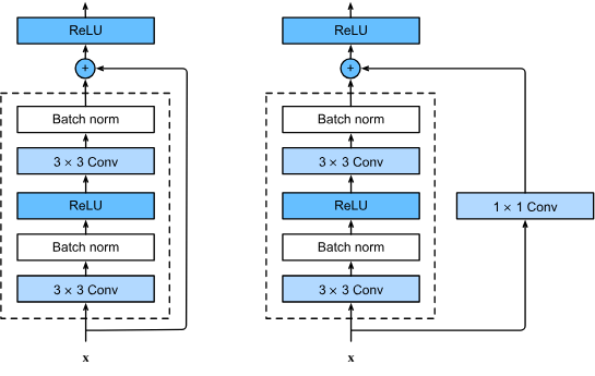
"Many intermediate transformations inside a very deep network are close to the identity. If one isn't, several residual blocks can compose many small residual changes into a large overall transformation"

So although the original intent was not to split up $f(x)$, we see we can split up $f(x) = \sum_{i} g_{i}(x) + x$ into many other blocks that each learn different parts. Before, these were just strictly learned as convolutional output channel features, but now there are much more expressive mappings that can be learned with non-linear $g(x)$ blocks

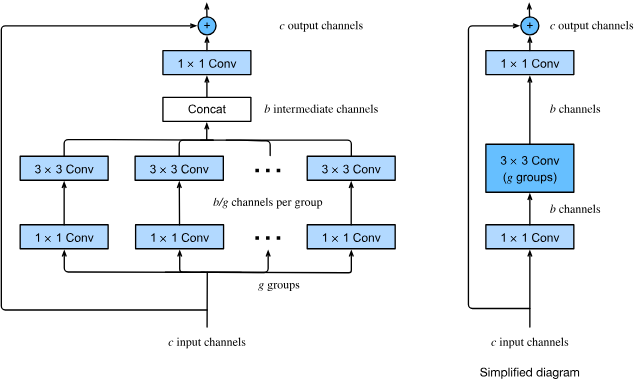
This does lead to a large quadratic runtime cost of $O(c_i \times c_o)$ because each input layer needs to be utilized for each output layer. 3 input channels and 6 outputs is 18 total calculations!

ResNet Vanishing Gradients

Since ResNets were presented as an answer to "can stacking more layers enable the network to learn better" - the obstacle up to that point fifn'y necessarily include vanishing / exploding gradients in a formal way. Most of the time they were primarily solved for by normalized initialization and intermediate batch normalization layers which enabled networks with tens of layers to start converging for stochastic gradient descent with backprop. Degredation was the main issue, where as network depth increased there was a saturation, and then rapid decrease, in accuracy. Adding more layers to a suitably deep model led to higher training error, and overfitting was not caused by this degredation. A shallower architecture was suggested, and using auxiliary layers consisting of identity mappings and others shallow model layers, but in practice this didn't help. Later on Deep Residual Learning took the charge, and utilized normalization / residual layers to help fix the problems of degredation.

The two were connected in some way, and solving for degredation did also help to solve the vanishing / exploding gradient problem via gradient highways that, when paired with batch normalization, allowed for non-degrading, converging gradients.

Parameters early on in CNN architectures sometimes don't receive meaningful gradient updates (vanishing gradients), sometimes the gradients are huge and chaotic (exploding gradients), the layers may not capture meaningful representations (just bad NN), or extra layers may degrade useful features in hidden layers (degredation)

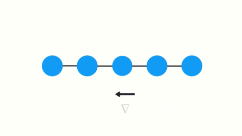
ResNets are an architecture that show promise in fixing many of the above issues, ultimately preserving gradients and allowing features to pass through downstream layers

Residual Learning (Again)

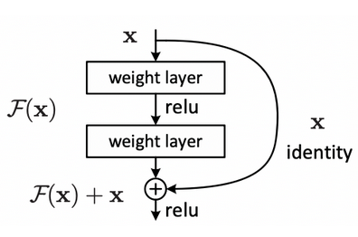
The idea of residual learning is to replace the approximation of an underlying latent mapping $H(x)$, which is approximated by a few stacked layers, with an approximation of residual functions $F(x) := H(x) - x$ where $x$ denotes the inputs to the first of these few stacked layers - therefore $H(x) \approx F(x) + x$

Below, the $F(x, {W_i})$ is the residual mapping that is to be learned, an example is $F = {W_2} \sigma ({W_1} x)$ in which $\sigma$ denotes the ReLU activation function - most experiments show that ID mapping is enough to solve the degradation problem

DenseNet

DenseNet, to some extent, is a logical extension of the ResNet architecture. DenseNet is characterized by both the connectivity pattern where each layer connects to all preceding layers and the concatenation operation (versus summing up the residual connections) to preserve and reuse features from earlier layers

ResNet decomposes functions into $f(x) = g(x) + x$, which can be viewed as a complex non linear term and a simple linear term. What if we wanted to capture information beyond two terms? And what if we wanted to capture non-additive information beyond two terms? The solution in 2017 was the DenseNet architecture

DenseNet Math Theory

The general intuition behind it is similar to Taylor Expansion at some point like $x = 0$

f(x) = f(0) + x \cdo [f^{'}(0) + x \cdot [f^{''}(0) \over {2!} + x \cdot [f^{'''}(0) \over {3!} + ...]]

The Taylor Expansion helps to approximate a complicated, messy function using simple polynomials. It matches the functions value, slope, and higher order curvature using derivatives. For a function $f(x)$ and a point $x = a$:

• The 0th derviative $f(a)$ is the constant term, and essentially just the $y$ height at that point. $y = f(a)$, we start things off directly at the function
• The 1st derivative $f^{'}(a)(x - a)$ allows us to find the slope at that point, and gives us a tangent line
• The second derivative gives us change of change, velocity, etc
• As more terms are added, the polynomial hugs the original function tighter and tighter over a larger internal
• We divide by $a!$ at each step to act as a counter-weight to remove the multiplication effects of repeatedly taking power-rule derivatives
• The further we open the interval $x$ around $a$, the more polynomials we need to help track where we'll go

Using these Taylor Expansions is much easier for computers to calculate versus sin(a) or something similar, and it's valid for a certain range around $a$. Calculators swap sin(a) for a 5th order polynomial to get a quick answer

DenseNet Concatenations

DenseNet doesn't do Taylor Series, but it reuses every possible skip connection it can, which ends up looking like a Taylor Series

Not every block is always a DenseBlock - DenseNet also uses $1 \times 1$ convolution layers known as TransitionLayers so that they don't create an exponentially increasing runtime model

EfficientNet

Before EfficientNet it was popular to scale only one of three dimensions - depth, width, or image size. Research papers and empirical studies, which ultimately led to EfficientNet, showed it's critical to balance all dimensions which can be achieved by scaling all 3 with a consistent ratio.

Compound Model Scaling

A function $Y_i = F_i(X_i)$ with operator $F_i$, output tensor $Y_i$, and input tensor $X_i$ of shape $(H_i, W_i, C_i)$ spatial dimensions $(H_i, W_i)$ and channel dimension $C_i$ is called a ConvNet Layer i

A ConvNet appears as a list of these composing layers $N = F_k \odot ... \odot F_2 \odot F_1(X_1)$

Effectively, these layers are often split / partitioned into multiple stages and all layers in each stage share the same architecture - an example is ResNet which has 5 stages ($k = 5$), with all layers in each stage being the same convolutional type except the first layer which performs down-sampling.

Scaling all 3 is important as they'r all fairly linked - you cannot increase the resolution of an image without increasing it's depth and saturation (idk what this means). Therefore, a compound scaling method which uniformly scales network width, depth, and resolution is required

Designing Convolutional Networks

Most of the convolutional networks above were heavily informed by human creativity, and less informed by systematic exploration of the design space. When you look up the choices behind each of these architectures, why they chose certain parameters, layer structures, and designs, most of it was just tweaking until loss converged. This network engineering approach was tremendously successful!

The other side of the coin would be neural architecture search (NAS) which is extremely expensive brute-force search with some forms of hyperparameter optimizations. EfficientNets are an outcome of this search type

Contrastive Learning

We've looked into Contrastive Learning in another sub-document, and will copy this section over there, but this is a section specifically on Image based Contrastive Learning

SlimCLR was one of the first, and most known, contrastive learning frameworks - it's simple, highly accurate, well researched, and heavily utilized. The main idea is to have two copies of a single image, and use these to train two networks that are compared. A major con is that it doubls the overall storage size of the underlying dataset, but BLOB storage is cheap (in my opinion). Boostrap Your Own Latent was introduced to avoid making the double sized dataset.

Contrastive Learning Framework

Contrastive loss is used to learn a representation by maximizing the agreement between various augmented views of the same data example. To achieve this, there are 4 significant components:

• A stochastic data augmentation module to create new augmentations of input
• A neural network base encoder to take inputs, and augmentations, and will encode into dense vector
• A small neural network projection head to take encoded vectors into projection space
• A contrastive loss function that allows comparisons between projected vectors

Stochastic Data Augmentation

A minibatch of $N$ examples is sampled randomly, and thee contrastive prediction task is defined on pairs of augmented examples - this results in $2N$ data points altogether

A memory bank isn't needed, as the training batch size varies from 256 to 8,192. Any given data example randomly returns two correlated views of the same example, denoted as $\bar{x_i}$ and $\bar{x_j}$ which is known as the positive pair. The negative pair are all other $2(N-1)$ pairs. It's been shown that choosing different data augmentation techniques can reduce the complexity of previous contrastive learning frameworks. Some of the common ones are:

• Spatial geometric transformations like cropping, resizing, roration, and cutouts
• Appearance transformations like color distortion, brightness, contrast, saturation, Gaussian blur, or Sorbel filtering

Models tend to improve after composing augmentaitons together too, instead of only applying one single one

Neural Network Base Encoder

The NN Base Encoder $f(\cdot)$ extracts multiple representation vectors from the augmented data examples - the commonly used ResNet was picked and gives $h_i = f(\bar{x_i}) = \text{ResNet}(\bar{x_i})$ where $\bold{h_i} \in \real^d$ is the output after the average pooling layer.

Small Neural Network Projection Head

A small neural network projection head $g(\cdot)$ maps the representation to the space where the contrastive loss is applied. The importance of this layer was evaluated with:

• Identity mapping
• Linear projection
• Default non-linear projection with an additional hidden layer and ReLU activation

The results showed the non-linear projection is better than linear, and both are much better than no transformation (identity)

They've used an MLP with one hidden layer to obtain $z_i = g(\bold{h_i}) = W^2 \sigma(W^1(\bold{h_i}))$ where $\sigma$ is a ReLU non-linear transformation

This is useful because defining the contrastive loss on $z_i$ instead of $\bold{h_i}$ wouldn't lead to a loss of information caused by contrastive loss, and is shown to maintain and form more information

Contrastive Loss Function

Given a set $\{{\bar{x}_{ik}}\}$ including a positive pair of examples $\bar{x_i}$ and $\bar{x_j}$, the contrastive prediction task aims to idntify $\bar{x_i}$ in $\{{\bar{x}_{i}}\}_{k \neq i}$ for a given $\bar{x_i}$. In the case of positive esxamples, the loss function is defined as

$\ell_{i,j} = -\log \frac{\exp\left(\frac{\mathrm{sim}(z_i, z_j)}{\tau}\right)}{\sum_{k=1}^{2N} \mathbb{I}[k \neq i] \exp\left(\frac{\mathrm{sim}(z_i, z_k)}{\tau}\right)}$

Where:

• $(\ell_{i,j})$ is the loss for the pair $(i, j)$
• $\mathrm{sim}(z_i, z_j)$ is the similarity between $z_i$ and $z_j$
  • Typically $\mathrm{sim}(u, v) = \frac{u^\top v}{|u| , |v|}$ is a dot product between $l_2$ and normalized $\bold{u}, \bold{v}$
• $\tau$ is the temperature parameter
• $\mathbb{I}[k \neq i]$ is the indicator function (1 if $(k \neq i)$, 0 otherwise)

The final loss is calculated across all positive pairs, both $(i, j)$ and $(j, i)$ in a mini-batch

This above was named NT-Xent as Normalized Temperature-scaled Cross Entropy. This was compared against other commonly used contrastive loss functions like logistic loss and margin loss, and NT-Xent outperformed with proper hyperparameter tuning

SlimCLR Framework

The ultimate goal of this framework was to describe a better approach to learning visual representations without human supervision.

SlimCLR outperforms previous work, is more straightforward, and does not require a memory banks

Significant components of the framework:

• A constrastive prediction task requires combining multiple data augmentation operations, which results in effective representations
  • Unsupervised contrastive learning benefits from more significant data augmentation
  • In english, this means applying lots of different random changes (like cropping, flipping, rotating, color changes, etc) to images. The model is trained to recognize that these different augmentations are "the same"
• The quality of learned representations can be substantially improved by introducing a learnable non-linear transformation between the representation and contrastive loss
  • Basically this means you encourage the model to make the representations (feature vectors) of different augmented views of the same image similar, while making representations of different images dissimilar
  • Contrastive loss will penalize the model is the two feature vectors of the same augmented image are far apart, and rewards them if they're similar
    • Common contrastive loss example is NT-Xent (Normalized Temperature-scaled Cross Entropy) loss
• Representation learning with cross-entropy loss can be improved by normalizing embeddings and adjusting the temperature parameter appropriately
  • Temperature is a parameter in the contrastive loss function that controls how sharply the model distinguishes between similar and dissimilar pairs
    • A lower temperature makes the model focus more on making positive pairs very close, and negative very far apart
    • A higher temperature smooths out the differences, making the model less strict about separating pairs
  • Therefore, this equates to saying that adjusting the temperature to balance how hard the model pushes similar images together can improve the quality of the learned representations
• Contrastive learning benefits from larger batch size and extended training periods compared to supervised counterpart
  • Larger batch size helps because it allows the model to compare more positives and negatives for each sample
  • Each batch is used to create positive and negative pairs, so the more examples inside of it the more comparisons!