LLM Training
LLM Training
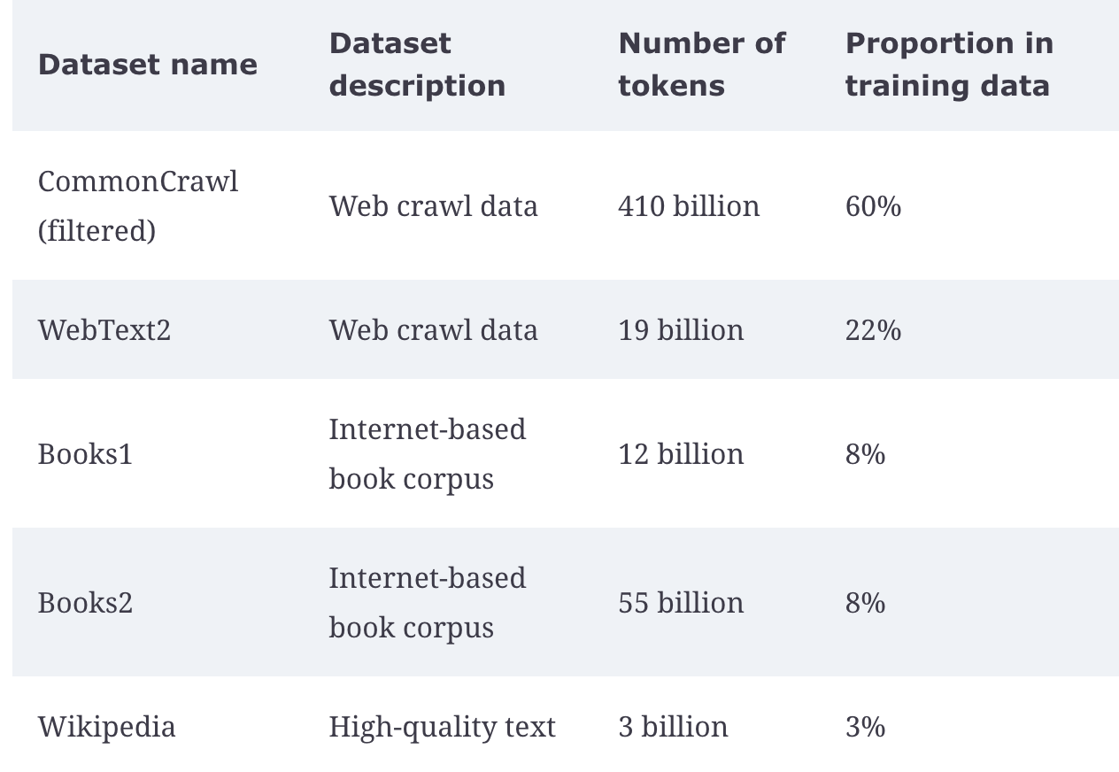
Various training datasets are used, mostly around sourced web content from social media, online encyclopedias, and structured curated text
LLM pipelines still rely heavily on tokenization models, embeddings, attention mechanisms, encoder-decoder interactions (or encoder / decoder only), and some regularization, dropout, and residual layers to ensure models are trained appropriately. Outside of that model evaluation utilizing BLEU scores
The general rule of thumb during training is 16GB of VRAM per 1 billion parameters
General Pipeline
Each of the architectures, encoder-decocer or only one or the other, have a fair amount of overlap given they all stem from transformers:
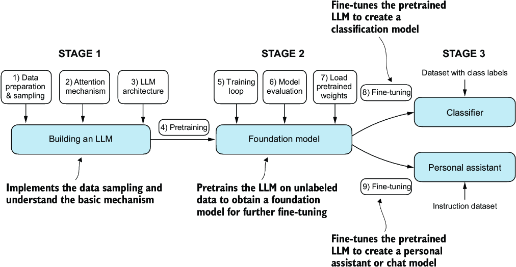
- (Pre)training steps are used to prep the models dataset, setup the model architecture, and decide on further layers and training tasks to ensure a model is able to achieve it's desired convergence. Afterwards, the actual training loop relies heavily on distributed compute, advanced hardware, and multiple evaluation rounds to check it's current convergence limits. Finally weights are stored, experiments logged, and the model is marked as a foundational ready model to run transfer learning on for any specific downstream task that's needed like classification, sentiment analysis, translation, etc
- (Pre)Training
- Data preparation and sampling
- Attention
- Further layers
- Foundational Model
- Training loop
- Evaluation
- Storage
- Distribution
- Model registries
- Transfer learning
Data Preparation And Sampling
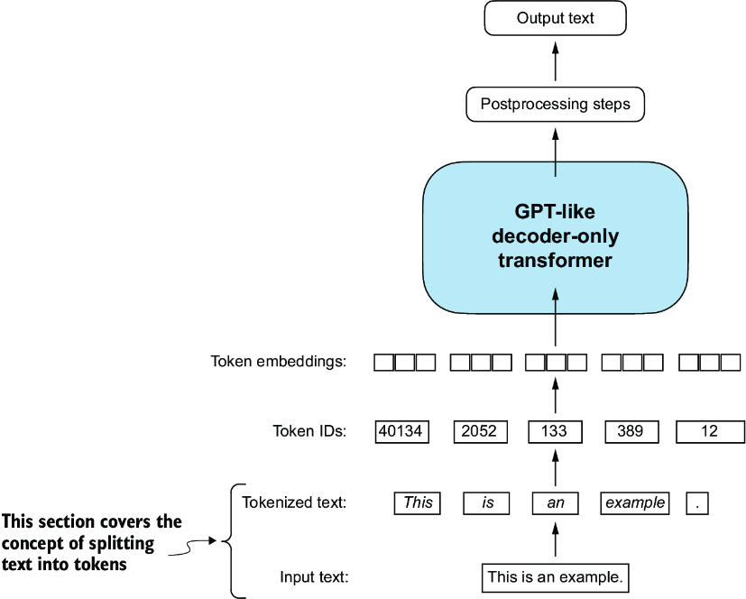
Data preparation involves sourcing, storing, and cleaning input data which comprises of massive datasets from the web, and then sending that data through initial model architectures so that it can be used by a transformer architecture
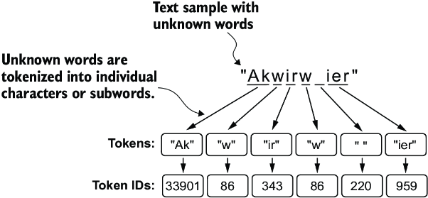
Datasets first need to be tokenized, which is essentially a compaction and extension process that allows the input dataset to be refined as a set of tokens that cover the entire span of potential future vocabulary. The general thought is, instead of creating embeddings for both rocking, rock, rocket, sock, socket, and socking, we might as well reuse a number of these sub-words as tokens instead. Some architectures use character-level tokens, but that means we only really have ~100 static embeddings, and it's difficult to glean any actual information about what these characters represent. Most modern day models utilize sub-word embeddings, and these are based on frequency counts and compaction procedures which are a sort of greedy algorithm. It is described further in the transformer subdocument, but it will produce tokens like rock, ##ing, sock, ##et which can then be concatendated / aggregated when 2 tokens are needed to combine to create a word like rocket. These models require their own complete training loop (which mostly means a few loops of greedy algorithms until convergence, not actual loss based ML models), and afterwards create a vocabulary of size for us to use. This hypothetically can extend to all future words, even ones we haven't seen yet (out-of-vocabulary) like yoloing, where the absolute furthest fall back is individual characters like [y, o, l, o, ##ing]. This means we don't have to constantly retrain the tokenization model for viral words or new phrases. The vocabulary itself will just have integers assigned to each of the tokens, and so for each token in future sequences we will look to find exact matches of those tokens, and worst case fall back to individual characters, and the ultimate output of this tokenization will be some way to lookup individual integers or embeddings for each token
- During training there will be batching performed, and so actual sequences may be of different sizes, and the shorter ones all need to have extra padding via
[PAD]tokens, and longer ones may be shrunk down to some specific size- Then, every input sequence is of the same size and can be sent through in a batch
- There are other special tokens used like
[BOS],[EOS], and[CLS]for marking beginning of sentences, ends, and places to classify or predict words
Character / token level ascii characters can't be used very well in neural networks, and so most actual computations are done on embeddings. The most well documented and "Hello oihgb
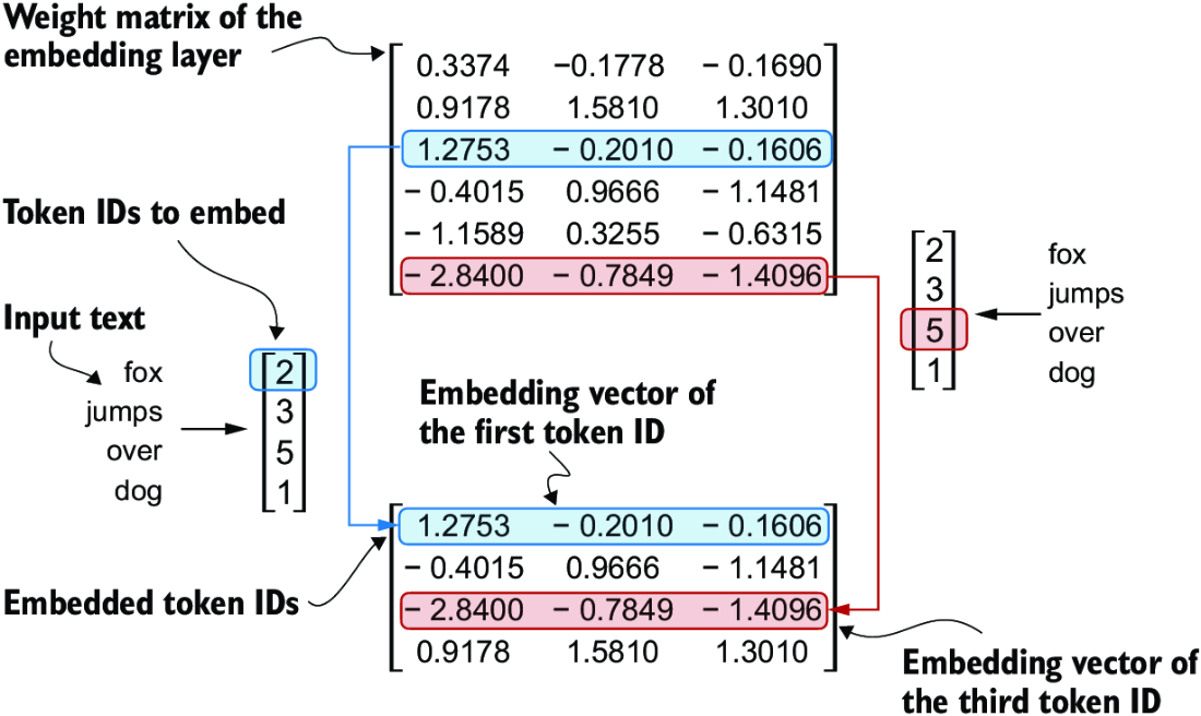
World" version of this is Word2Vec, which creates static embeddings for each token in the input vocabulary by utilizing a bag-of-words or skip-gram architecture for predicting context words / missing single words in the training dataset to come up with a compressed representation of size for each of the input tokens. Typically this is size 128, 256, 512, or 1024. These embeddings are static, and so the river bank and the bank teller, both bank instances here have the same underlying embedding representation. Most LLM systems come up with their own embeddings during training, and don't reuse foundational vocabularies like those in Word2Vec. A key point on the examples below is most of them are pulling integer values for the tokens, which are actually just used as lookups to actual embedding vectors, so the input to the model is actually a sequence of embedding vectors of size for each token in the input sequence, and these are then sent through the rest of the model architecture. The embedding layer is essentially a lookup table that takes in the integer token IDs and outputs their corresponding embedding vectors, which are then fed into the subsequent layers of the model
At this point the first ~2 layers of any LLM are usually covered, there are some other layers such as positional encodings that are used to encode the position of the token in the sequence
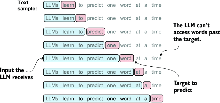
During training next token prediction is the usual task, along with next sentence prediction, masked language modeling, and other similar tasks. The loss function is usually some form of cross-entropy loss, and the model is trained to minimize this loss across the training dataset. Sliding window sampling is the method used to create each of these pairs of input and output sequences, where we take a window of size and slide it across the input sequence to create multiple training examples. For example, if we have a sequence of tokens [the, cat, sat, on, the, mat] and a window size of 3, we would create training examples like:
- Input:
[the, cat, sat], Output:on - Input:
[cat, sat, on], Output:the - Input:
[sat, on, the], Output:mat
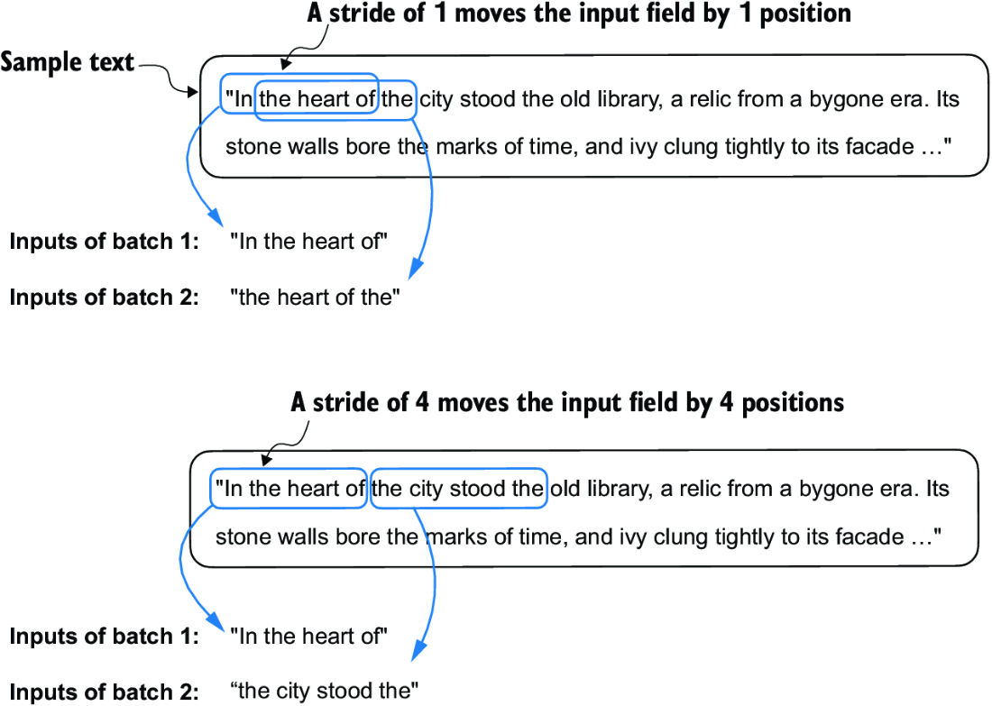
The main parameters in sliding window are:
- Window size: The number of tokens in the input sequence (e.g., 3 in the example)
- Stride: The number of tokens to move the window each time (e.g., 1 in the example, which means we move the window one token at a time)
TikToken Tokenizer + Sampling
from tiktoken import TikTokenizer
tokenizer = TikTokenizer()
text = (
    "Hello, do you like tea? <|endoftext|> In the sunlit terraces"
     "of someunknownPlace."
)
encoded = tokenizer.encode(text, allowed_special={"<|endoftext|>"})
print(encoded)
# [15496, 11, 466, 345, 588, 8887, 30, 220, 50256, 554, 262, 4252, 18250,
#   8812, 2114, 286, 617, 34680, 27271, 13]

strings = tokenizer.decode(encoded)
print(strings)

# Hello, do you like tea? <|endoftext|> In the sunlit terraces of
#   someunknownPlace.

# Sliding Window
context_size = 4         #1
x = encoded[:context_size]
y = encoded[1:context_size+1]
print(f"x: {x}")
print(f"y:      {y}")

for i in range(1, context_size+1):
    context = enc_sample[:i]
    desired = enc_sample[i]
    print(context, "---->", desired)

# [290] ----> 4920
# [290, 4920] ----> 2241
# [290, 4920, 2241] ----> 287
# [290, 4920, 2241, 287] ----> 257
#  and ---->  established
#  and established ---->  himself
#  and established himself ---->  in
#  and established himself in ---->  a
This is all great theory, but the actual training of models requires large scale iterators ran over distributed compute. The actual training pipeline should use a distributed training framework like PyTorch's Distributed Data Parallel (DDP) or TensorFlow's MirroredStrategy to parallelize the training across multiple GPUs or even multiple machines. These allow us to write some general pipeline code, and then MirroredStrategy will take care of the distribution and synchronization of gradients across the different devices. The training loop itself will involve iterating over the training dataset, computing the loss, and updating the model weights using an optimizer like Adam or SGD. Writing synchronization code across potentially failing hardware during training loop runs would take months of work, testing, and planning. Instead of doing that, just reuse the community tested and used frameworks!
These frameworks utilize autoloaders and iterators to handle data loading and batching. Under the hood most of the iterators run as generators which yield batches of data to the training loop, and these batches are then sent to the appropriate devices for training. The frameworks also handle the synchronization of gradients across devices, which is crucial for ensuring that the model converges properly during training
Torch Data Loader
import torch
from torch.utils.data import Dataset, DataLoader
class GPTDatasetV1(Dataset):
    def __init__(self, txt, tokenizer, max_length, stride):
        self.input_ids = []
        self.target_ids = []

        # Tokenize the actual text
        token_ids = tokenizer.encode(txt)

        # Use a sliding window to chunk the
        #  sequence into overlapping sequences of max_length
        for i in range(0, len(token_ids) - max_length, stride):
            input_chunk = token_ids[i:i + max_length]
            target_chunk = token_ids[i + 1: i + max_length + 1]
            self.input_ids.append(torch.tensor(input_chunk))
            self.target_ids.append(torch.tensor(target_chunk))

    # Get total n rows
    def __len__(self):
        return len(self.input_ids)

    # Get a single row from the dataset
    def __getitem__(self, idx):
        return self.input_ids[idx], self.target_ids[idx]

def create_dataloader_v1(txt, batch_size=4, max_length=256,
                         stride=128, shuffle=True, drop_last=True,
                         num_workers=0):
    # Initialize tokenizer and dataset
    tokenizer = tiktoken.get_encoding("gpt2")
    dataset = GPTDatasetV1(txt, tokenizer, max_length, stride)
    dataloader = DataLoader(
        dataset,
        batch_size=batch_size,
        shuffle=shuffle,
        # drop_last=True drops the last batch if it is shorter than the
        #   specified batch_size to prevent loss spikes during training
        drop_last=drop_last,
        # The number of
        #   CPU processes to use for preprocessing
        num_workers=num_workers
    )

    return dataloader

# Dummy input text
with open("file.txt", "r", encoding="utf-8") as f:
    raw_text = f.read()

torch.manual_seed(123)
vocab_size = 50257
output_dim = 256
max_length = 4
context_length = max_length

dataloader = create_dataloader_v1(
    raw_text, batch_size=8, max_length=max_length,
    stride=max_length, shuffle=False
)
# Generator that yields batches of data from the dataloader
data_iter = iter(dataloader)
inputs, targets = next(data_iter)

token_embedding_layer = torch.nn.Embedding(vocab_size, output_dim)
token_embeddings = token_embedding_layer(inputs)
pos_embedding_layer = torch.nn.Embedding(context_length, output_dim)
pos_embeddings = pos_embedding_layer(torch.arange(context_length))
input_embeddings = token_embeddings + pos_embeddings
For each of the batches for our sliding window, we can setup window size, stride, and batch size as needed. After this, each of the batches can be padded to the same length, and sent through the model for training. A batch size of 32 will result in 32 sequences of dimensional embeddings with 32 corresponding target sequences / labels
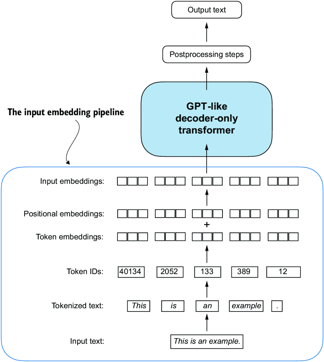
Finally, most of the embeddings also require positional encodings, which are added to the token embeddings to give the model information about the position of each token in the sequence. This is crucial for the model to understand the order of the tokens, which is important for tasks like language modeling and translation. The positional encodings can be either learned or fixed, and they are typically added to the token embeddings before being fed into the transformer layers. Positional encoding structure and in depth choices are discussed more in that Transformers sub-document
All of the code sits in /docs/llm_systems/code/data_prep.py, and it's actually fairly straightforward:
data_loadergets an encoder class and sets up all objects to pass into a dataset classGPTDatasetV1GPTDatasetV1creates an iterator that returns slices of token input indexes and target indexes that are used to create inputs and labels- Looping over this with
gpt_dataset.next()lets us pull in data over time from gigantic datasets without overwhelming local memory - We ingest
batch_size x stride_lengthfrom the data loader- It's creating the inputs as
input_chunk = token_ids[i:i + max_length] target_chunk = token_ids[i + 1: i + max_length + 1]- It's step size is based on stride
for i in range(0, len(token_ids) - max_length, stride): - So altogether, it'll jump
strideindexes at each step, and then if ourmax_lengthis four and we're at index 3, it'll pull3-7for inputs and targets as4-8 - This is still next token prediction, where the model will try to predict tokens
4, then5, then6, etc...- Input: [the, cat, sat]
- Target: [cat, sat, on]
- The model is trained to predict each token in the target sequence based on the corresponding input sequence, and the model can predict all tokens in target sequence simultaneously in parallel
- It should look to predict
catforthe,satforcat, andonforsat
- This is exactly what we see when stepping through functions:
>>> print(inputs, targets)tensor([[ 40, 367, 2885, 1464], ....tensor([[ 367, 2885, 1464, 1807], ....
- It's creating the inputs as
- This will then go through both token and positional embeddings, which will get added together to create the final input embeddings
- Input is size
[8, 4]of batch size 8 and context size 4 as described above - Input embedding layer defined as
Embedding(vocab_size, output_dim)which represents the50257vocab size and our output dimension of 256 - Once we do
embedding_layer(input)it needs to somehow convert an8x4matrix into8x4x256matrix representing each input records tokens embedding. If an input record is 4 words, we need an embedding for each word, i.e.8x4x256 - The actual matrix indexing and lookup operations would need to be
inp = 8x4- The embedding weight matrix is size
vocab x output_dim - Each input token needs to be indexed in the embedding weight matrix which returns a size
256embedding - These are stacked together
- It's not actually matrix multiplication for this part, it's some indexing and stacking in parallel behind the scenes
- Input is size
- Add this to the positional embeddings which are
pos_embeddings.size() >>> torch.Size([4, 256])- Input is 8 batches of
4x256 - Positional is only
4x256 - So this addition is done via broadcasting which allows tensors of different shapes to be added together as long as their dimensions are compatible
- These broadcasting rules are figured out by automatically expanding dimensions of smaller tensors to match larger tensors shape, as long as the dimensions are compatible:
- If dimension is
1or missing, it's expanded to match the corresponding dimension of larger tensor
- If dimension is
- These broadcasting rules are figured out by automatically expanding dimensions of smaller tensors to match larger tensors shape, as long as the dimensions are compatible:
- So since the 8 dimension is missing, the
4x256is expanded (copied) 8 times to matchinput_embeddingsand we just add the positional to each one- I do think this is incorrect, on purpose, because if our positional embeddings are created via
torch.arange()and come out to[0, 1, 2, 3, 4], our inputs are- tokens at
[0, 1, 2, 3, 4]with targets[1, 2, 3, 4, 5] - but the next rows have stride
- The next row in batch is
[0+stride, 1+stride, 2+stride, 3+stride], with targets[1+stride, 2+stride, 3+stride, 4+stride], and so adding the static positional embeddings here would be incorrect - Need to update positional embeddings to include stride
- tokens at
- I do think this is incorrect, on purpose, because if our positional embeddings are created via
- Input is 8 batches of
- Looping over this with
So overall, the final preparation, tokenization, and embedding layers will result in a number of input layers below, and during training there's sliding, window size, and generation considerations for us to produce the actual input and training labels
- LLMs require textual data to be converted into numerical vectors, known as embeddings, since they can’t process raw text. Embeddings transform discrete data (like words or images) into continuous vector spaces, making them compatible with neural network operations
- As the first step, raw text is broken into tokens, which can be words or characters. Then, the tokens are converted into integer representations, termed token IDs
- Special tokens, such as
<|unk|>and<|endoftext|>, can be added to enhance the model’s understanding and handle various contexts, such as unknown words or marking the boundary between unrelated texts - The byte pair encoding (BPE) tokenizer used for LLMs like GPT-2 and GPT-3 can efficiently handle unknown words by breaking them down into subword units or individual characters
- We use a sliding window approach on tokenized data to generate input–target pairs for LLM training
- Embedding layers in PyTorch function as a lookup operation, retrieving vectors corresponding to token IDs. The resulting embedding vectors provide continuous representations of tokens, which is crucial for training deep learning models like LLMs
- While token embeddings provide consistent vector representations for each token, they lack a sense of the token’s position in a sequence. To rectify this, two main types of positional embeddings exist: absolute and relative. OpenAI’s GPT models utilize absolute positional embeddings, which are added to the token embedding vectors and are optimized during the model training
Attention Mechanisms
There are many many many types of attention, such as:
- Self attention
- Simplified, regular, and optimized
- Causal self attention, which is a simplified version that allows a model to consider only previous and current inputs in a sequence, ensuring temporal order during text generation
- Multi-head attention which extends self attention and causal attention and enables a model to simultaneously attend to information from different representation subspaces (heads)
The reason that self-attention is so useful, is that historic attempts to store context over long sequences ultimately degraded. RNN's are sequential and reuse a context vector , which had limitations on total context storage over long sequences. Also grammar styles between languages like engligh and spanish aren't 1:1 and sequential, many instances of words need to be re-arranged with 1:M or M:1 mappings. Because of this, most NN's use two submodules, encoders and decoders. For short sequences, RNN architectures work completely fine, but for longer ones the accuracy starts to degrade with each new token
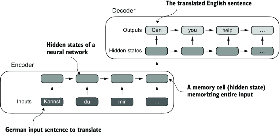
Bahdanau Attention was a relatively newer attempt (2014) to overcome this and allowed decoders to directly access encoder hiddens states at each step, and ultimately helped it bypass long sequence lengths for providing context, but it was still sequential in nature
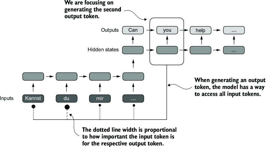
Atferwards, the transformer architecture showcased the self-attention architecture which showed that RNN architecture wasn't required for building these deep NN's. Self-attention allows each token in the input sequence to consider the relevancy of, or attend to, all other positions in the same sequence when computing the embedding of a sequence. Decoder only models like GPT, encoder only models like BERT, and encoder-decoder models like T5 all utilize self-attention in different places whether it's encoding input embeddings or auto-regressively predicting output words in decoder. The goal of self-attention is to compute a context vector for each input token that combines information from all other input elements
Parameters and dimensions:
- Input
- = Sequence length
- = Model dimension
- = # of heads
- = /
- Projection matrices , ,
GPT_CONFIG_124M = {
    "vocab_size": 50257,     # Vocabulary size
    "context_length": 1024,  # Context length
    "emb_dim": 768,          # Embedding dimension
    "n_heads": 12,           # Number of attention heads
    "n_layers": 12,          # Number of layers
    "drop_rate": 0.1,        # Dropout rate
    "qkv_bias": False        # Query-Key-Value bias
}
Simple Self Attention
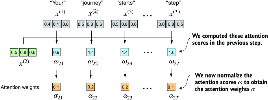
This implementation looks to create a simplified variant of self-attention without any trainable weights - it will cover a similar concept as the alignment score in self-attention
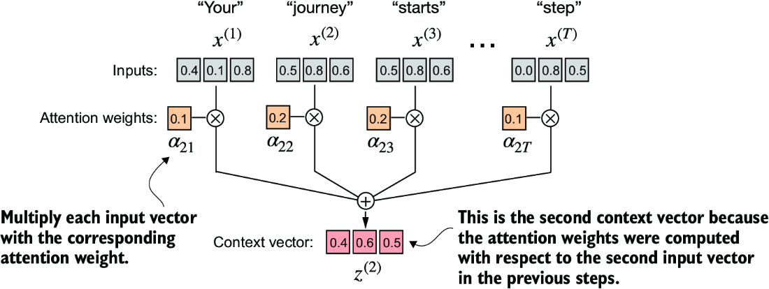
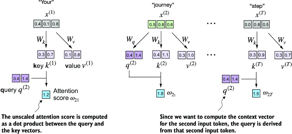
The goal here should be to produce alignment scores which described the key effect on our query , and aggregate them together to come up with a context vector which is the overall affect of each input token . Each element of the sequence, such as , corresponds to a dimensional embedding vector representing a specific token, and so ultimately this results in us just comparing a to every , finding some comparison metric , and then finding the overall alignment over each of them via softmax / normalization before aggregating into the vector
So doing this in torch would involve some torch.dot, some for i, x_i in inputs: and a few other items, which are easy enough. The real goal of this is to figure out how we can parallelize the entire thing so that it can be done via efficient matrix multiplication
attn_scorewill correspond to score vectorattn_weightsrefer to the softmax normalized scores, and we do this along each row (dim = -1will run over last dimension, if we have[row, col]it would normalize over cols so that sum across a row equals 1)all_context_vecswould then have the final contextually attended to vectors, where we are shifting the input vector by some amount via each other input
Simplified Self Attention
attn_scores = inputs @ inputs.T
attn_weights = torch.softmax(attn_scores, dim=-1)
all_context_vecs = attn_weights @ inputs
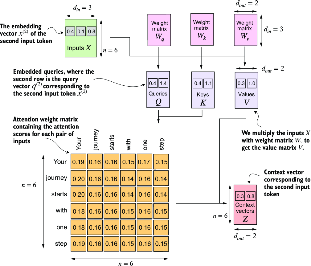
Scaled Dot Product Attention
This self-attention is what most folks think of when utilizing self-attention. It involves matrices for altering the initial input embeddings, and will also utilize some scaling and normalization dimensions to ensure gradients don't explode or vanish
Since we have projection matrices , , , and our input , the result of for any of the
attn_scorescan still be calculated by comparing keys to queriesattn_weightsneeds to continue performing softmax, but there's a new scaling parameter involved- This is the square root of the embedding dimension, and actually helps to avoid small gradients. When the embedding dimensions are huge, a large dot product can result in very samll gradients during back propogation due to the softmax function applied to them, and so as the dot product becomes larger the softmax behaves more like a step function resulting in gradients nearing zero
- Scaling by the square root of the dimension ensures that these dot products don't grow too large, which sort of brings them back to center to ensure proper updates can still be made
Scaled Dot Product Attention
import torch.nn as nn
class SelfAttention(nn.Module):
    def __init__(self, d_in, d_out, qkv_bias=False):
        super().__init__()
        # nn.Linear has more stable weight init schema compared
        #   to nn.Parameter(torch.rand(d_in, d_out))
        self.W_query = nn.Linear(d_in, d_out, bias=qkv_bias)
        self.W_key   = nn.Linear(d_in, d_out, bias=qkv_bias)
        self.W_value = nn.Linear(d_in, d_out, bias=qkv_bias)

    def forward(self, x):
        keys = self.W_key(x)
        queries = self.W_query(x)
        values = self.W_value(x)
        attn_scores = queries @ keys.T
        attn_weights = torch.softmax(
            attn_scores / keys.shape[-1]**0.5, dim=-1
        )
        context_vec = attn_weights @ values
        return context_vec

torch.manual_seed(123)
sa_v1 = SelfAttention(d_in, d_out)
print(sa_v1(inputs))
Masked Attention
Masked attention, also known as causal attention is self-attention which considers only tokens that appear prior to the current position when predicting the next token in a sequence
It's often used in the transformer decoder phase, and decoder only GPT style LLMs. For each token processed, it just needs to mask future tokens because during inference it won't have access to future tokens as they don't exist and will be generated
During the softmax operations we still need to ensure that our rows add up to 1, and there's a few other considerations to ensure things can be ran in parallel without screwing up the operations
- During training we compute attention in the same parallel format over all context tokens, then we zero out the upper triangle, and recompute the softmax over only the bottom triangle
- This does in fact nullify the effects of future words on our current word. They don't contribute to the softmax score in any meaningful way - i.e. the distribution of attention weights is as if it was calculated only among the unmasked positions to begin with
keys = self.W_key(x)
queries = self.W_query(x)
values = self.W_value(x)
attn_scores = queries @ keys.T
attn_weights = torch.softmax(
    attn_scores / keys.shape[-1]**0.5, dim=-1
)
context_length = attn_scores.shape[0]
mask_simple = torch.tril(torch.ones(context_length, context_length))

# This is to renormalize the attention
#   weights to sum up to 1
masked_simple = attn_weights*mask_simple
row_sums = masked_simple.sum(dim=-1, keepdim=True)
masked_simple_norm = masked_simple / row_sums
This can be sped up by tricking the softmax function and using -inf values in our mask, as they're effectively treated as 0's by softmax functions, which removes the need for a good portion of code above, and allows us to continue with the simple implementation that's parallelized
mask = torch.triu(torch.ones(context_length, context_length), diagonal=1)
masked = attn_scores.masked_fill(mask.bool(), -torch.inf)
attn_weights = torch.softmax(masked / keys.shape[-1]**0.5, dim=1)
context_vec = attn_weights @ values
Masked Attention With Dropout
Dropout is a technique where randomly selected hidden layer units are ignored during training, effectively dropping them out. This is ultimately used to prevent overfitting by ensuring a model does not become overly reliant on any specific set of hidden layer units - this is only used during training
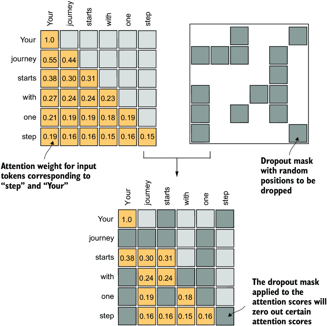
Remember, at the end of attention it's just an output of the same number of input tokens with an attended to set of weights versus static embeddings, so if we use dropout on top of this it's essentially just removing some dimensions of the embedding at the end. Pytorch provides this implementation with a dropout rate, where you specify the portion of units you'd want dropped torch.nn.Dropout(0.5)
During masked self attention, we only allow the vectors to the left to attend to the embeddings, but the effect is still the same. You only allow some of the words to be included in the embedding. To ensure the overall balance of attention weifhts are maintained, we scale up the existing weights by 1 / \text{dropout_rate}. This is handled automatically by the torch implementation
There are a few differences, but nothing major:
- Utilizing dropout layers, which handle batch inputs and scaling automatically
- Register buffer of dropout which essentially caches them in GPU memory for fast access
masked_fill_showcases the suffix_operations from pytorch, which perform operations in-place and avoid unnecessary memory copies- Everything else is similar, where we have outputs:
[batch_size, n_input_tokens, embedding_output_dim_size]
Masked Attention
import torch.nn as nn
class SelfAttention(nn.Module):
    def __init__(self, d_in, d_out, qkv_bias=False):
        super().__init__()
        # nn.Linear has more stable weight init schema compared
        #   to nn.Parameter(torch.rand(d_in, d_out))
        self.W_query = nn.Linear(d_in, d_out, bias=qkv_bias)
        self.W_key   = nn.Linear(d_in, d_out, bias=qkv_bias)
        self.W_value = nn.Linear(d_in, d_out, bias=qkv_bias)

    def forward(self, x):
        keys = self.W_key(x)
        queries = self.W_query(x)
        values = self.W_value(x)
        attn_scores = queries @ keys.T
        attn_weights = torch.softmax(
            attn_scores / keys.shape[-1]**0.5, dim=-1
        )
        context_vec = attn_weights @ values
        return context_vec

class MaskedAttention(nn.Module):
    def __init__(self, d_in, d_out, context_length,
                dropout, qkv_bias=False):
        super().__init__()
        self.d_out = d_out
        self.W_query = nn.Linear(d_in, d_out, bias=qkv_bias)
        self.W_key   = nn.Linear(d_in, d_out, bias=qkv_bias)
        self.W_value = nn.Linear(d_in, d_out, bias=qkv_bias)
        self.dropout = nn.Dropout(dropout)
        self.register_buffer(
           'mask',
           torch.triu(torch.ones(context_length, context_length),
           diagonal=1)
        )

    def forward(self, x):
        b, num_tokens, d_in = x.shape
        keys = self.W_key(x)
        queries = self.W_query(x)
        values = self.W_value(x)

        attn_scores = queries @ keys.transpose(1, 2)
        attn_scores.masked_fill_(
            self.mask.bool()[:num_tokens, :num_tokens], -torch.inf)
        attn_weights = torch.softmax(
            attn_scores / keys.shape[-1]**0.5, dim=-1
        )
        attn_weights = self.dropout(attn_weights)

        context_vec = attn_weights @ values
        return context_vec

torch.manual_seed(123)
sa_v1 = SelfAttention(d_in, d_out)
print(sa_v1(inputs))

context_length = batch.shape[1]
ca = CausalAttention(d_in, d_out, context_length, 0.0)
context_vecs = ca(batch)
# torch.Size([2, 6, 2])
# batch size of 2, 6 input tokens, and output is an embedding
#   of size 2
print("context_vecs.shape:", context_vecs.shape)
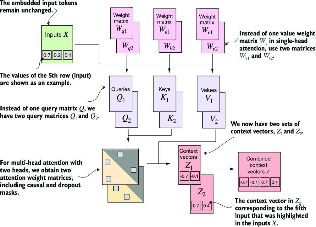
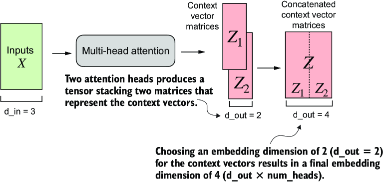
Multi Head Attention
Extending masked attention to multiple heads, aka multi-head attention, mostly means utilizing multiple matrices that are all updated, pushing them all through self-attention and masked attention, and then concatenating the results
The easiest way to do this is simply by utilizing multiple attention modules above, as they all will effectively encompass the parts of each attention set . At the end we basically just concatenate all of the output resulting vectors of size
Masked Attention
import torch.nn as nn
class SelfAttention(nn.Module):
    def __init__(self, d_in, d_out, qkv_bias=False):
        super().__init__()
        # nn.Linear has more stable weight init schema compared
        #   to nn.Parameter(torch.rand(d_in, d_out))
        self.W_query = nn.Linear(d_in, d_out, bias=qkv_bias)
        self.W_key   = nn.Linear(d_in, d_out, bias=qkv_bias)
        self.W_value = nn.Linear(d_in, d_out, bias=qkv_bias)

    def forward(self, x):
        keys = self.W_key(x)
        queries = self.W_query(x)
        values = self.W_value(x)
        attn_scores = queries @ keys.T
        attn_weights = torch.softmax(
            attn_scores / keys.shape[-1]**0.5, dim=-1
        )
        context_vec = attn_weights @ values
        return context_vec

class MaskedAttention(nn.Module):
    def __init__(self, d_in, d_out, context_length,
                dropout, qkv_bias=False):
        super().__init__()
        self.d_out = d_out
        self.W_query = nn.Linear(d_in, d_out, bias=qkv_bias)
        self.W_key   = nn.Linear(d_in, d_out, bias=qkv_bias)
        self.W_value = nn.Linear(d_in, d_out, bias=qkv_bias)
        self.dropout = nn.Dropout(dropout)
        self.register_buffer(
           'mask',
           torch.triu(torch.ones(context_length, context_length),
           diagonal=1)
        )

    def forward(self, x):
        b, num_tokens, d_in = x.shape
        keys = self.W_key(x)
        queries = self.W_query(x)
        values = self.W_value(x)

        attn_scores = queries @ keys.transpose(1, 2)
        attn_scores.masked_fill_(
            self.mask.bool()[:num_tokens, :num_tokens], -torch.inf)
        attn_weights = torch.softmax(
            attn_scores / keys.shape[-1]**0.5, dim=-1
        )
        attn_weights = self.dropout(attn_weights)

        context_vec = attn_weights @ values
        return context_vec

class MultiHeadAttentionWrapper(nn.Module):
    def __init__(self, d_in, d_out, context_length,
                 dropout, num_heads, qkv_bias=False):
        super().__init__()
        self.heads = nn.ModuleList(
            [MaskedAttention(
                 d_in, d_out, context_length, dropout, qkv_bias
             )
             for _ in range(num_heads)]
        )

    def forward(self, x):
        return torch.cat([head(x) for head in self.heads], dim=-1)

torch.manual_seed(123)
context_length = batch.shape[1] # This is the number of tokens
d_in, d_out = 3, 2
mha = MultiHeadAttentionWrapper(
    d_in, d_out, context_length, 0.0, num_heads=2
)
context_vecs = mha(batch)

print(context_vecs)
# torch.Size([2, 6, 4])
# represents the batch size 2, with 6 input tokens each,
#   of size 4, which is equal to output_dim * n_heads
#   because we concatenate them
print("context_vecs.shape:", context_vecs.shape)
This is great! But there's a for loop, i.e. it's not parallelized, which can be solved by slapping them together and doing matrix multiplication! We can also just completely collapse the multi-head wrapper with the masked attention module, and even collapse in self attention:
- Self attention is just a specific implementation of masked attention with
masking = False - Masked attention is a specific implementation of multi-head attention with
n_heads = 1 - To ensure input and output dimensions are kept, we need to track the dimensions of each head
head_dim output_projis a linear layer to combine the head outputs- weight matrices still have the same size and dimensions in the forward pass
- These are reshaped and transposed with
.viewandtranspose, and then computesattn_scorein the same way as usual 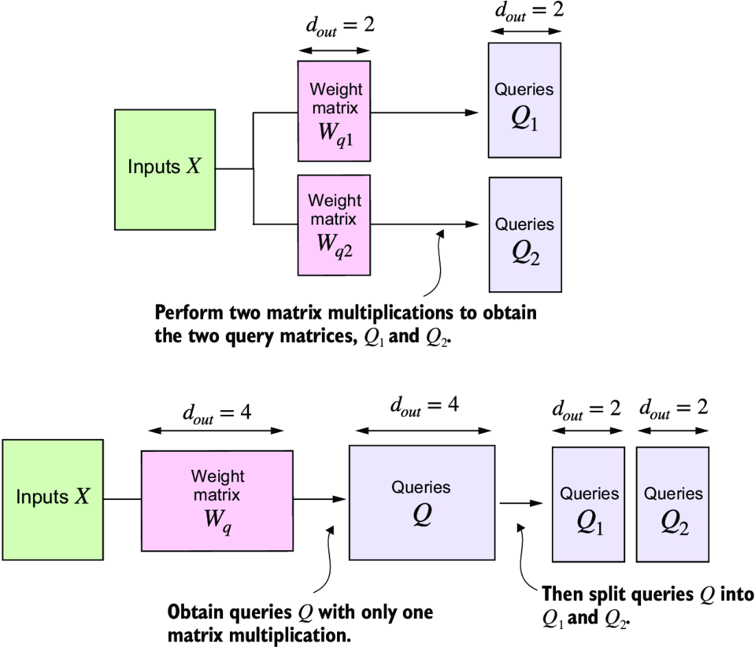
- These are reshaped and transposed with
- The important dimensionality part to focus on is
head_dim = d_out / n_headswhich splits the final output size, which was 4 above when we had 2 heads, and divide it by the number of heads to get each heads total dimension- After that splitting things up with
.viewmethod is essentially split out inton_headsdistinct matrices from(batch_size, input_tokens_size, d_out)to dimension(batch_size, input_tokens_size, n_heads, head_dim) - This is then transformed into
(batch_size, n_heads, input_tokens_size, head_dim), moving then_headspart forward, which allows for transposing with the same vector transposing the last 2 dimensions- This part is just something you need to sit at a computer and step through and debug there's no good way to describe it without seeing it
- Just want to be sure the
(input_tokens_size, head_dim)is the part we are doing matrix multiplication on, as that represents a(6, 2)matrix from our previous example and is our ideal "unit" to perform attention on
- After that splitting things up with
- Stacking and flattening the vectors together is then done to mimic the wrapper class, and finally an output projection layer is commonly used (but not implemeneted below)
Why is this more efficient? Calling of keys = self.W_key(x), and Q / V as well, is only done once and not on a per-wrapper call. This is usualy one of the most expensive steps
Merged Attention
class MultiHeadAttention(nn.Module):
    def __init__(self, d_in, d_out,
                 context_length, dropout, num_heads, qkv_bias=False):
        super().__init__()
        assert (d_out % num_heads == 0), \
            "d_out must be divisible by num_heads"

        self.d_out = d_out
        self.num_heads = num_heads
        self.head_dim = d_out // num_heads
        self.W_query = nn.Linear(d_in, d_out, bias=qkv_bias)
        self.W_key = nn.Linear(d_in, d_out, bias=qkv_bias)
        self.W_value = nn.Linear(d_in, d_out, bias=qkv_bias)
        self.out_proj = nn.Linear(d_out, d_out)
        self.dropout = nn.Dropout(dropout)
        self.register_buffer(
            "mask",
            torch.triu(torch.ones(context_length, context_length),
                       diagonal=1)
        )

    def forward(self, x):
        b, num_tokens, d_in = x.shape
        keys = self.W_key(x)
        queries = self.W_query(x)
        values = self.W_value(x)

        keys = keys.view(b, num_tokens, self.num_heads, self.head_dim)
        values = values.view(b, num_tokens, self.num_heads, self.head_dim)
        queries = queries.view(
            b, num_tokens, self.num_heads, self.head_dim
        )

        keys = keys.transpose(1, 2)
        queries = queries.transpose(1, 2)
        values = values.transpose(1, 2)

        attn_scores = queries @ keys.transpose(2, 3)
        mask_bool = self.mask.bool()[:num_tokens, :num_tokens]

        # ignore for full self-attention
        attn_scores.masked_fill_(mask_bool, -torch.inf)

        attn_weights = torch.softmax(
            attn_scores / keys.shape[-1]**0.5, dim=-1)
        attn_weights = self.dropout(attn_weights)

        context_vec = (attn_weights @ values).transpose(1, 2)

        # combine heads
        context_vec = context_vec.contiguous().view(
            b, num_tokens, self.d_out
        )
        context_vec = self.out_proj(context_vec)
        return context_vec

torch.manual_seed(123)
batch_size, context_length, d_in = batch.shape
d_out = 2
mha = MultiHeadAttention(d_in, d_out, context_length, 0.0, num_heads=2)
context_vecs = mha(batch)
print(context_vecs)
print("context_vecs.shape:", context_vecs.shape)
The smallest GPT-2 model has 12 attention heads and d_out of 768, while the largest has 25 attention heads and d_out of 1,600!
These attention mechanisms transform input elements into enhanced context vector representations that incorporate information about all inputs
Decoder Transformer Blocks
Decoder only models like GPT-3 only use the decoder portion, and are trained on massive datasets using solely a next word prediction task
They still focus on auto-regressive decoder-only architecture, and ultimately utilizing the next word / sentence prediction means the 400 billion token input dataset can be re-used almost infinitely
These LLM's take a large amount of the above architecture and combine it with further transformer layers like normalization, shortcuts, residuals, and non-linear layers to ultimately create a GPT style model that avoids vanishing / exploding gradients, create non-linear features, and ultimately move forward with creating human text
GPT models are built on top of multi-headed attention built into transformer blocks
New layers to create transformer blocks:
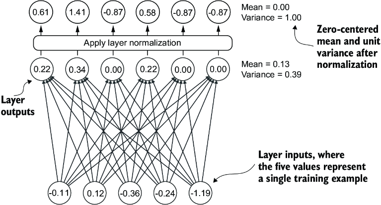
- Normalization Layer: This will take a vector input and normalize the weights. It'll find mean and variance for each input sequence of tokens, and normalize the activations based on those, which ensures each the input to each layer afterwards has a stable distribution
- GELU Activation: A non-linear activation function that acts as a smooth alternative to ReLU. It'll combine aspects of dropout, zoneout, and ReLU
- Segments out inputs based on magnitude, not strictly based on sign like ReLU does
- Feed Forward Network: Simple feed-forward layer(s) to give model more expressive power
- Shortcut Connections: Will bring results from residual layers through to further downstream layers
- AKA Residual connections
Dummy GPT Model
import torch
import torch.nn as nn

class DummyGPTModel(nn.Module):
    def __init__(self, cfg):
        super().__init__()

        # Input embeddings
        self.tok_emb = nn.Embedding(cfg["vocab_size"], cfg["emb_dim"])
        self.pos_emb = nn.Embedding(cfg["context_length"], cfg["emb_dim"])

        # Dropout config to reuse
        self.drop_emb = nn.Dropout(cfg["drop_rate"])

        # Sequential transformer blocks
        self.trf_blocks = nn.Sequential(
            *[DummyTransformerBlock(cfg)
              for _ in range(cfg["n_layers"])]
        )
        self.final_norm = DummyLayerNorm(cfg["emb_dim"])

        # Output layer to project from final transformer block
        self.out_head = nn.Linear(
            cfg["emb_dim"], cfg["vocab_size"], bias=False
        )

    def forward(self, in_idx):
        batch_size, seq_len = in_idx.shape
        tok_embeds = self.tok_emb(in_idx)
        pos_embeds = self.pos_emb(
            torch.arange(seq_len, device=in_idx.device)
        )
        x = tok_embeds + pos_embeds
        x = self.drop_emb(x)
        x = self.trf_blocks(x)
        x = self.final_norm(x)
        logits = self.out_head(x)
        return logits

class DummyTransformerBlock(nn.Module):    #3
    def __init__(self, cfg):
        super().__init__()

    def forward(self, x):     #4
        return x

class DummyLayerNorm(nn.Module):           #5
    def __init__(self, normalized_shape, eps=1e-5):    #6
        super().__init__()

    def forward(self, x):
        return x
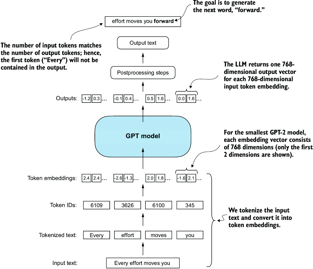
Out of the box, if we tokenize 2 sentences with tiktoken and send them through, we will get an output of [2, 4, 50257] which corresponds to 2 sentences, each of 4 words, with ~50k predictions for each element in the vocabulary. I.e. we haven't created any of the postprocessing code, so this is basically just a giant softmax over the vocabulary for the predicted next word
tokenizer = tiktoken.get_encoding("gpt2")
batch = []
txt1 = "Every effort moves you"
txt2 = "Every day holds a"

batch.append(torch.tensor(tokenizer.encode(txt1)))
batch.append(torch.tensor(tokenizer.encode(txt2)))
batch = torch.stack(batch, dim=0)

torch.manual_seed(123)
model = DummyGPTModel(GPT_CONFIG_124M)
logits = model(batch)
print("Output shape:", logits.shape)
print(logits)
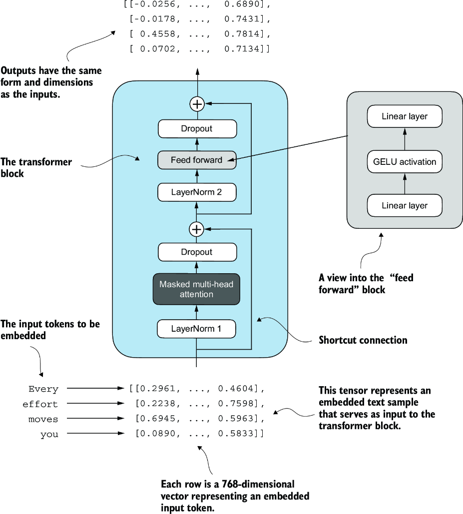
At the end, the idea is to combine all of the below layers to create transformer blocks. Ultimately, the tokens input into the model are sent through these transformer blocks to transform these input vectors in a way that preserves dimensionality and allows us to predict the next token! Attention mechnisms identity and analyze relationships between elements in the input sequence, feed forward blocks modified individual data points at each position, and skip connections ensure gradients don't vanish. This enables more nuanced understanding from the model, and allows the model to have an overall larger capacity for handling complex data patterns. Preserving dimensionality allows stacking of multiple blocks on top of each other without having to manually tweak any parameters or dimensions
Normalization Layers
During training there are often issues with vanishing and exploding gradients - these are created by multiplying together hundreds, thousands, or millions of floating point numbers together which will either explode outwards, or converge to 0 (vanishing). Overall it's just from unstable training dynamics which make it difficult for the network to effectively adjust its weights over time, and so minimizing the loss function is incredibly slow or sometimes impossible
The main goal of layer normalization is to adjust the activations (outputs) of a NN layer to have a mean of 0 and variance of 1, i.e. unit variance. This ultimately just speeds up convergence to effective weights by ensuring consiste, reliable distributions. Doing this is just subtracting mean and dividing by square root of variance
Layer normalization is different from batch normalization which normalizes across the batch dimension. Layer norm normalizes across the feature dimension. LLM's have a huge amount of computational overhead, and so hardware / memory constraints may reduce the overall batch size - layer normalization can ensure normal distributions in a single row or in a batch, independent of batch size
class LayerNorm(nn.Module):
    def __init__(self, emb_dim):
        super().__init__()
        # Need an epsilon so that it's not explicitly 0
        self.eps = 1e-5
        self.scale = nn.Parameter(torch.ones(emb_dim))
        self.shift = nn.Parameter(torch.zeros(emb_dim))

    def forward(self, x):
        mean = x.mean(dim=-1, keepdim=True)
        # Bessel correction (unbiased)
        var = x.var(dim=-1, keepdim=True, unbiased=False)
        norm_x = (x - mean) / torch.sqrt(var + self.eps)
        return self.scale * norm_x + self.shift
These layers are typically applied before and after multi-head attention modules
GELU Activations
Historically ReLU activation functions were used due to simplicity and effectiveness, but Gaussian Error Linear Unit (GeLU) was chosen in a large number of modern day LLM's. They are more complex, smoother, and offer improved performance for deep learning models. The "sharpness" of ReLU can lead to some issues with optimizations, and GeLU will allow for a small non-zero output for negative values which still allows these neurons to contribute to training process
Theoretically it should be implemented as:
Where is the cumulative distribution function of standard gaussian - there's a much cheaper implementation specified in GPT-2 paper
class GELU(nn.Module):
    def __init__(self):
        super().__init__()

    def forward(self, x):
        return 0.5 * x * (1 + torch.tanh(
            torch.sqrt(torch.tensor(2.0 / torch.pi)) *
            (x + 0.044715 * torch.pow(x, 3))
        ))
Feed Forward Network
GeLU layers are often combined with LinearLayer that can double or triple the size of the embeddings. This is mostly used to ensure uniformity in dimensions (inputs and outputs of linear blocks are same size for stacking multiple blocks) while allowing for an overall larger and "richer" feature space for the model to use

Shortcut Connections
Shortcut connections, AKA residual or skip connections, were first introduced in Residual CNN Networks, AKA Resnets. They allow information from earlier layers to be reused in downstream layers, and ultimately are used as a way to help solve for vanishing gradient problems. They allow the larger gradients to pass through where they may have been lost with all of the small floating point operations
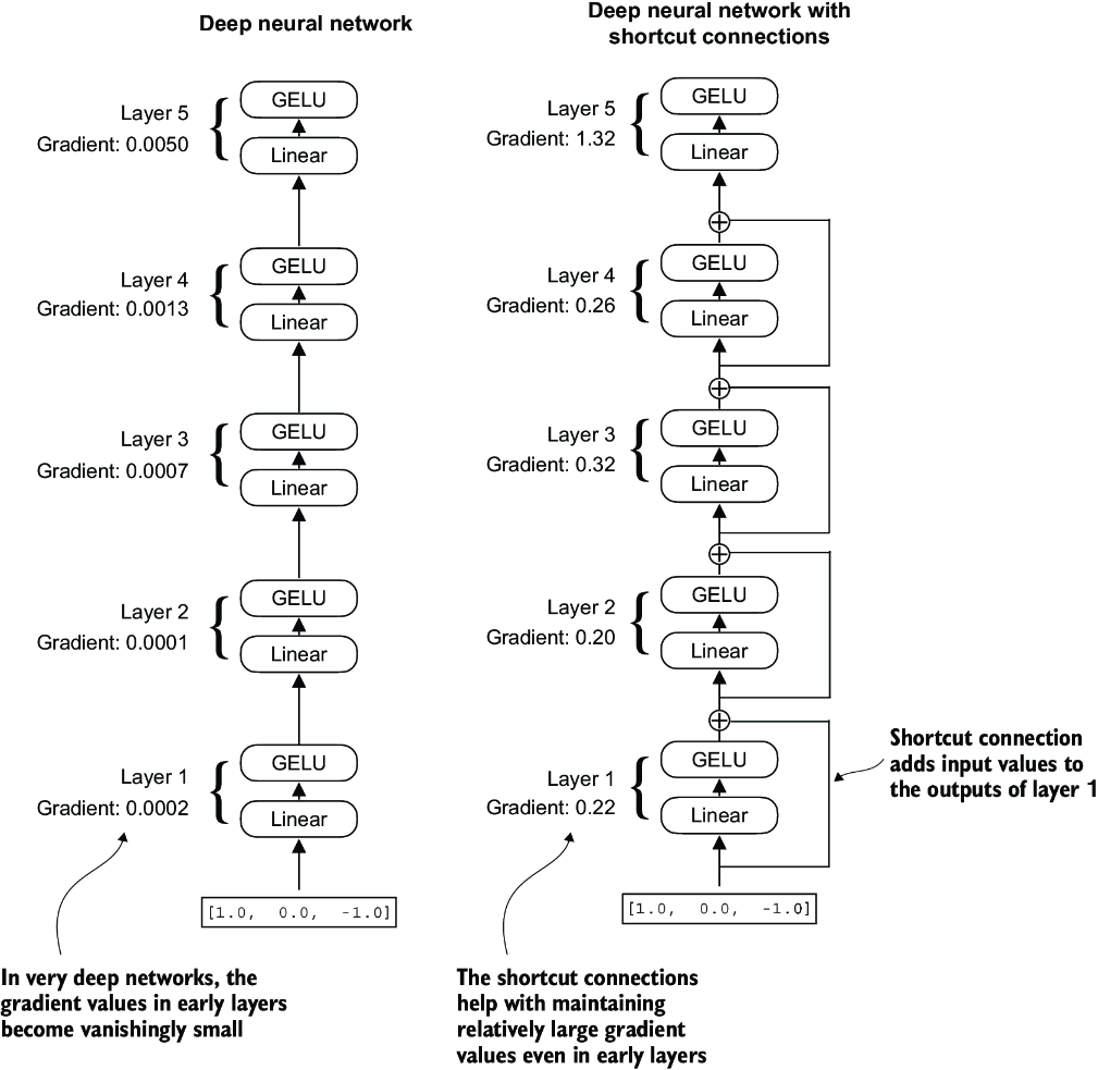
As an example, if you create a small NN with a few Feed Forward layers without skip connections and you print out the gradient at each layer via .backward() call paired with loss, you can see it decrease over each layer...with enough layers you get vanishing gradients. Skip connections are proven time after time to keep these layers gradients larger, which may lose some information / be inefficient, but ensures gradients don't vanish. Thinking through it, if we pass in gradients from the initial layer it means we are just taking those gradients as "true" and letting them flow down even though gradients partial derivatives may be more nuanced at the further layers...it's definitely a trade-off, but the nuanced further layers do alter the gradient themselves so they aren't lost completely
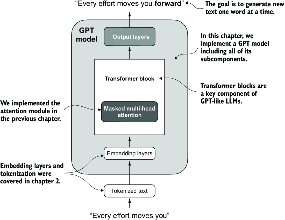
GPT Model
At this point implementing a GPT-2 style model can be done with most of the layers defined above!
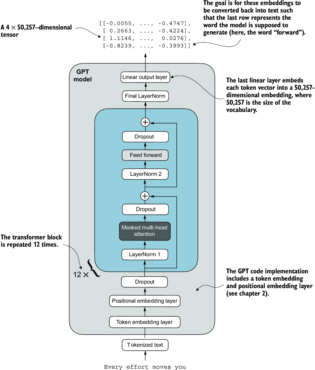
An overview of the GPT model architecture showing the flow of data through the GPT model. Starting from the bottom, tokenized text is first converted into token embeddings, which are then augmented with positional embeddings. This combined information forms a tensor that is passed through a series of transformer blocks shown in the center (each containing multi-head attention and feed forward neural network layers with dropout and layer normalization), which are stacked on top of each other and repeated 12 times
Real GPT-2 Model
class TransformerBlock(nn.Module):
    def __init__(self, cfg):
        super().__init__()
        self.att = MultiHeadAttention(
            d_in=cfg["emb_dim"],
            d_out=cfg["emb_dim"],
            context_length=cfg["context_length"],
            num_heads=cfg["n_heads"],
            dropout=cfg["drop_rate"],
            qkv_bias=cfg["qkv_bias"])
        self.ff = FeedForward(cfg)
        self.norm1 = LayerNorm(cfg["emb_dim"])
        self.norm2 = LayerNorm(cfg["emb_dim"])
        self.drop_shortcut = nn.Dropout(cfg["drop_rate"])

    def forward(self, x):
        shortcut = x
        x = self.norm1(x)
        x = self.att(x)
        x = self.drop_shortcut(x)
        x = x + shortcut

        shortcut = x
        x = self.norm2(x)
        x = self.ff(x)
        x = self.drop_shortcut(x)
        x = x + shortcut
        return x

class GPTModel(nn.Module):
    def __init__(self, cfg):
        super().__init__()
        self.tok_emb = nn.Embedding(cfg["vocab_size"], cfg["emb_dim"])
        self.pos_emb = nn.Embedding(cfg["context_length"], cfg["emb_dim"])
        self.drop_emb = nn.Dropout(cfg["drop_rate"])

        self.trf_blocks = nn.Sequential(
            *[TransformerBlock(cfg) for _ in range(cfg["n_layers"])])

        self.final_norm = LayerNorm(cfg["emb_dim"])
        self.out_head = nn.Linear(
            cfg["emb_dim"], cfg["vocab_size"], bias=False
        )

    def forward(self, in_idx):
        # embeddings
        batch_size, seq_len = in_idx.shape
        tok_embeds = self.tok_emb(in_idx)

        # device id just sets CPU or GPU
        pos_embeds = self.pos_emb(
            torch.arange(seq_len, device=in_idx.device)
        )
        x = tok_embeds + pos_embeds
        x = self.drop_emb(x)

        # pass input through transformer blocks
        x = self.trf_blocks(x)

        # final last norm
        x = self.final_norm(x)

        # logits represent probabilities of words
        #  - should be size vocab
        logits = self.out_head(x)
        return logits

torch.manual_seed(123)
model = GPTModel(GPT_CONFIG_124M)

out = model(batch)
print("Input batch:\n", batch)
print("\nOutput shape:", out.shape)
print(out)
GPT-2 Specific Choices
There are some specific nuanced choices GPT-2 makes:
- Weight tying reuses the initial token embedding weights in the final output layer, as the
~50kvocab size is a large part of memory- This is worse off in terms of accuracy and training, but creates a smaller model memory footprint
Choosing A Next Token - Generating Text
The output of the model above is ~50k logit probabilities - how can we choose the actual next word?
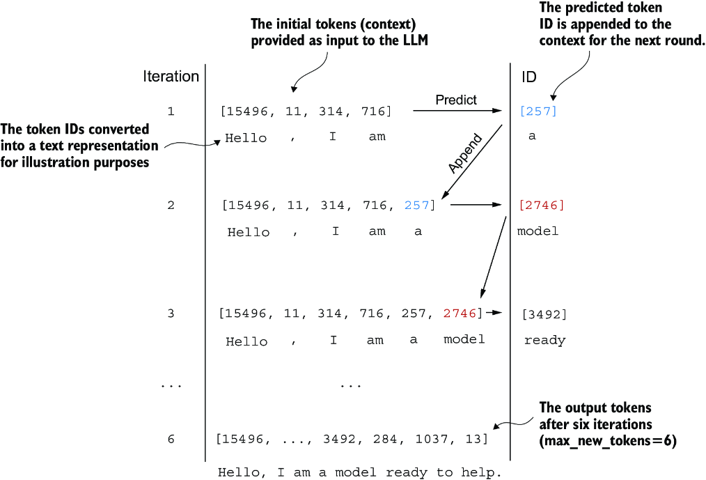
Greedy decoding, i.e. picking the "most probably" is a valid option, but typically isn't the most accurate long term. Most models have some sort of beam search portion that let's the model follow a top-k generative output path to see which one results in the best sequence
Maximizing the probability of the final sequence isn't equivalent to maximizing the probability of the next best token
Architectures
Multiple architectures, all used for diff things and probably covered elsewhere
Encoder Only
Encoder only models like BERT are trained for masked language modeling. Actual BERT training information is stored in that page, but will go more in depth here
TODO