Graph Neural Networks

Graph NN

Graph's as a concept are defined in the [Graph DSA Topic](/docs/dsa/8. trees & graphs/index.md)

Graph Neural Networks (GNN's) can be directly applied to graph data structures, and provide a way to leverage the relationships and connections between nodes for machine learning tasks

GNN's can operate on the graph level, node level, edge level, or even subgraph level - most of the same common tasks are still used in GNN's such as classification, regression, clustering, imputation, and link prediction

Graphs are typically stored in adjacency matrices, so there's no specific need to do anything special outside of typical matrix deep learning over matrices, but other times graphs are stored as lists of neighbors and traversing means iterating over all edges in total (i.e. neighbors of an unseen node)

• A dense adjacency matrix gives immediate access to linear algebra style operations (matrix multiplications) that can exploit highly efficient and optimized parallel computations
• A dense matrix is memory-intensive for large sparse graphs, where it stores a large amount of zero's, when compared to adjacency lists / edge lists
  • An adjacency matrix stores $O(v^2)$ space, where adjacency lists store $O(v + e)$ space

Ideally, graph calculations can reuse concepts from linear algebra over matrices, without storing large sparse matrices with redundant information

In the real world implementations, a majority of graphs are stored as sparse matrices using efficient formats that don't store all the zero entries explicitly, such as Compressed Sparse Row (CSR) or Compressed Sparse Column (CSC) formats, or as an edge list (two arrays of source / target indices). These formats still allow for linear algebra benefits, like running parallel linear algebra operations over them, or they utilize parallel graph traversal frameworks like GraphX or Pregel

GraphX and Pregel allow for massively parallel operations in tools like Spark, while utilizing edge list storage formats

Early Days - CNN's Over Graphs

In the past CNN's were tried over Graphs where you take convolutions over sub-graphs of nodes - CNN's worked well on images, so the thought was that it should be like using CNN over an image with some missing pixels

Pooling layers, convolutions, subsampling, etc allow for CNN's to perform image classifiction, object detection, and many other tasks on images - ultimately fueled by their ability to capture local spatial hierarchies in data

This sliding window approach was thought to be generalizable to graphs as well, but the complex topology of graphs restricts this - images are more rigid with well defined dimensions, whereas graphs can have arbitrary structures and varying node degrees

Moving forward, GNN's have taken more of a message passing / aggregation approach, where nodes aggregate information from their neighbors to update their own representations - this is the core idea behind many GNN and Parallel Graph Processing frameworks like GraphX and Pregel

Basics of Graph Neural Networks

Thinking about graph ML, can you still view it as supervised, unsupervised, contrastive, etc? Well, yes, you can, but a lot of the old ML tasks like regression, classification, and segmentation aren't portable over to graphs because underlying data assumptions typically can't port over to a graph

There are no independent and identically distributed (i.i.d) distributions, and data is no longer independent at all (vertices are, but edges aren't?)

The main difference is something called homophily, which is the tendency for nodes to share attributes with their neighbors in the graph

From this, there are other Graph Statistics, Sub-Graph Statistics such as Eigencentrality, and Vertex Statistics

• Eigencentrality is a core theoretical underpinning that PageRank and other centrality / ranking graph algorithms used in their initial setup
  • PageRank, hypothetically, could assign important nodes (webpages) in the internet based on their centrality rank (this would ignore user queries, but we could serve the "most central internet page")
• Eigenvectors as a whole have a whole slew of things they can help uncover in graphs such as stable distributions, node important, community detection, network dynamics, etc - these sorts of analysis don't even require neural nets, they just need linear algebra
  • Large eigenvalues indicate an overall interconnected and influential network (as a whole)
  • Dominant eigenvectors provide insights into the most significant vertices inside of a graph, higher magnitudes indicate higher centrality and importance
  • Eigenvectors associated with smaller (non-dominant) eigenvalues acn be used for community detection or identifying sub-graphs (neighborhoods)
  • Algebraic connectivity of a graph's Laplacian can indicate the connectivity or presence of bridges in the network
  • Node rankings can be found via the eigenvector relating to the largest eigenvalue - the higher the rank (value) of the entry, the more influential the node

Some online articles mention different types of graph learning, but realistically they are just 2 different types of machine learning overall:

• Transductive Learning: Solves a specific problem by leveraging both training and test data together. If test node features and adjacency are available during training $\rarr$ transductive
  • In graph problems, it means the full graph, including nodes we'll predict later on, are known at training time
  • You still learn embeddings for those unknown nodes, and at test time you reveal labels for the unknown nodes in the test set
    • This means the unknown nodes can still influence embeddings of other nodes during training
• Inductive Learning: Generalizes from training data to unseen data, making predictions on new nodes or graphs. If test nodes / graphs appear only after training (no adjacency seen) $\rarr$ inductive
  • You must produce embeddings for nodes (or entire sub-graphs), not seen during training - they are net new and arrive after training and weight updates
• Common examples and their types:
  • GraphSAGE is more aimed towards inductive, where you can create embeddings on net new nodes that arrive after training, specifically without retraining
  • Link prediction can be both
    • Transductive when we predict missing edges in known graphs, or reveal edges in graphs
  • Whole graph classification is typically inductive, where the model generalizes to classify unseen graphs

Graph Kernel Methods

Graph Kernel Methods are classes of ML algorithms that can be used to learn from data that's represented as a graph to create statistics, embeddings, features, or other tasks on top of graphs (or sub-graphs by extension)

Graph kernel methods define similarity between whole graphs or sub-structures by utilizing non-parametric methods

Other Graph Neural Networks like Node Embedding and Classification are parametric methods, and so they are outside of the scope here

For example the Bag Of Nodes graph kernel method will create a graph embedding by simply utilizing a permutation invariant function over all of the vertices in a graph, such as concatenation, averaging, summation, etc. Since vertices are just vectors, combining them is a valid way of embedding a graph! The Weisfeiler-Lahman method will take the dot product of all of the vectors

Neighborhood overlap detection is also technically a graph kernel method which answers the question of "which pair of nodes are related based on their similarities" - similar to the Word2Vec example of King - Man + Woman = Queen, where (King, Man) is probably related to (Queen, Woman)

Random Walk Methods

Random walk–based methods matter because they connect graph structure to Markov chain theory (PageRank, DeepWalk, Node2Vec, spectral clustering)

A stationary distribution in a Markov Chain is a long run equilibrium of a random process, and it can also be useful to identify steady-state behaviors in graphs

The stationary distribution of a (finite, irreducible, aperiodic) Markov chain gives long‑run visit frequencies; on a simple random walk over a connected, non‑bipartite undirected graph it is proportional to node degree. In english, this means that a random walk method is proportional to node degree (given the graph has certain characteristics and no "missing bumps")

If you take a random walk around a graph starting at $v$ and end up, eventually, at $u$, then there exists some path between the two nodes and means they're in the same connected component

The stationary distribution, $\pi$, is a single global vector, $\pi P = \pi$, that gives long-run visit frequencies. Therefore, long run visit probabilities between nodes are entries of $P^t$, Figuring out the long term stationary distribution from every node to every other node is a similar idea to finding the transition probabilities, and long run stationary distribution, in a Markov Chain - and can be formalized as powers of the transition matrix

Therefore, graph random walk methods can be understood through the lens of Markov chains, providing insights into node connectivity, graph structure, and visiting probabilities

The TLDR of the article below is that the similarity between a pair of nodes is based on how likely they are to visit eachother Random Walk Method - Page Rank Algorithm using NetworkX

Node Embedding

One of the most common GNN tasks is Node Embedding - where each node in the graph is mapped to a low-dimensional vector space, capturing both the node's features and its structural context within the graph with a goal of mapping similar nodes to nearby points in the embedding space. Similarity in the embedding space should approximate similarity in the graph structure or node attributes

The task at hand is to learn a function $f: V \rightarrow \mathbb{R}^d$ that maps each node to a $d$-dimensional embedding vector - typically, it utilizes operations like:

• Convolutional layers
  • These convolutional layers consists of graph convolutions that aggregate information from a node's neighbors, and different layers or functions can be used to capture different aspects of the graph structure
    • Can aggregate only a slice of neighbors, all neighbors, certain radius neighbors, etc
• Pooling layers
• Fully connected layers
• Attention mechanisms
• Non-linear activations
• Normalization layers
• Parameter learning
  • Typical backpropogation, gradient descent, SGD, Adam, etc
• Loss functions
  • These are typically designed to encourage similar nodes to have similar embeddings, such as contrastive loss, triplet loss, cross-entropy loss for classification tasks, reconstruction loss for autoencoder setups
• etc..

A fair amount of node embeddings are done via encoder-decoder methodologies, where the encoder maps nodes to embeddings and the decoder reconstructs graph properties or predicts tasks based on these embeddings. The encoder operates on input graph data, which will be adjacency list or edge list and node feature matrix. For an encoder to create meaningful features, it will use tools from above like aggregating and transforming node attributes, incorporating neighborhood information via message passing, or potentially some combination of the two

After this is done the decoder is meant to map the latent embeddings back out to graph structures for different tasks - it can do edge prediction (link prediction), attribute prediction, or other graph-related tasks. Loss functions depend on the task type, so the typical ML techniques of choosing your loss based on task still are valid here

Outside of these methods we can also see contrastive architectures where we mask some of the known inputs and try to recreate them after the decoder output, ultimately utilizing contrastive loss functions to test if our embeddings capture this information. This helps with datasets where there aren't specific supervised learning tasks and we still want embeddings and other prediction tasks as output.

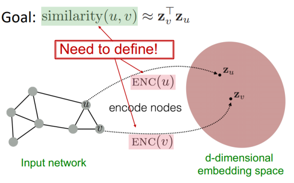
For this $u$ and $v$ are nodes in the graph, and $z_u = f(u)$ and $z_v = f(v)$ are their respective embeddings. The goal is to minimize a loss function that encourages similar nodes to have similar embeddings - setup would have something like $\text{similarity}(u, v) \approx z_v^T z_u$

The encoder function should be able to:

• Perform locality (local network neighborhood) calculations
• Aggregate information from neighboring nodes
• Stack multiple layers (compute across multiple hops)

Ultimately, the similarity $S(z_u, z_v)$ should be high for similar nodes and low for dissimilar ones, and during inference time this similarity score would be output for all relationships and we'd do threshold tuning and typical precision / recall trade-offs for link prediction, attribute prediction, or other tasks

Most of these 3 things can be achieved by utilizing graph traversal algorithms, implemented via message passing in scalable parallel frameworks, to aggregate information from neighbors and update node representations. Perhaps the most common way to do this is through neighborhood aggregation, where each node aggregates information from its immediate neighbors to update its own representation

After this is done the decoder reconstructs graph properties or predicts tasks based on these embeddings. Loss functions can help us optimize the embeddings to be useful for downstream tasks, where we compare what the decoder predicted for edges, node

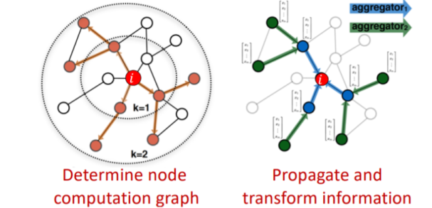
The locality information can be preserved through message passing, and neural networks can help facilitate the aggregation and transformation of node features during this process - neural networks allow information to be aggregated across layers in a linear and non-linear fashion, simply by doing linear algebra operations. In below freehand NN's are represented by gray boxes, which shows how we can represent a graph as linear transformations over dynamic inputs

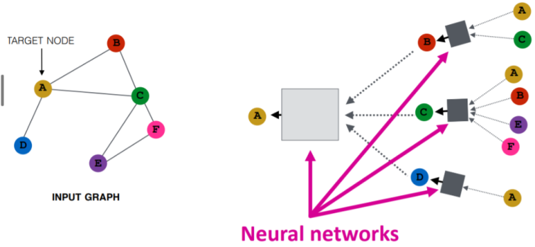
The dynamic input sizes are a problem, if you alter the above representation to one that's more "NN-like", you can achieve the below freehand - it showcases how a Graph NN architecture can be transformed into a feedforward NN architecture

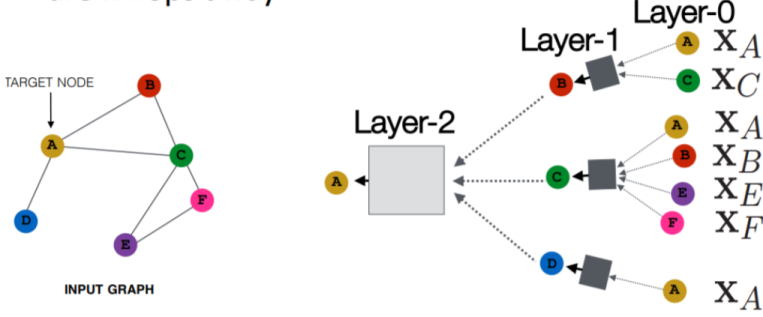
In the above diagram:

• Each node has a feature vector - $(X_A)$ is the feature vector of node $A$
• The inputs are the feature vectors, and a gray box takes the inputs and applies a linear transformation, aggregates them, and passes them forward to the next layer
  • In Layer-0 above, the input size to the gray boxes is dynamic (some nodes have more or less connections than others)
  • To handle this, the aggregation function needs to be permutation invariant, such as sum, mean, or max, ensuring consistent output size regardless of the number of neighbors

In the forward propagation steps we'd have:

1. Initialize node features: $h_v^{(0)} = X_v$ for each node $v$.
2. For each layer $k = 1, \dots, K$:
   • Neighborhood aggregation (mean): $\bar{h}_v^{(k)} = \frac{1}{|N(v)|} \sum_{u \in N(v)} h_u^{(k-1)}$
     • This equates to "averaging the feature vectors of all neighbors of node $v$ at the previous layer"
     • This layer is permutation invariant, ensuring consistent output size regardless of the number of neighbors - 2 neighbors or 100 neighbors result in same output size
   • Update / combine self and neighborhood: $h_v^{(k)} = \sigma\big( W_k \bar{h}_v^{(k)} + U_k h_v^{(k-1)} + b_k \big)$
     • $W_k$ weights for neighbor messages; $U_k$ self-feature weights; optional bias $b_k$
     • $\sigma$ any non-linearity (e.g. ReLU)
     • We merge the aggregated neighbor information $\bar{h}_v^{(k)}$ with the prior embedding $h_v^{(k-1)}$, which already encodes up to $(k\!- 1)$-hop information
       • Stacking layers expands the receptive field: after $k$ layers, $h_v^{(k)}$ depends (under mean aggregation) on nodes up to $k$ hops away
       • This depth-wise accumulation is analogous in spirit to RNN hidden states carrying context, but the model is still a feed-forward stack
         • It still "drags along" information, but it happens via feed forward NN
       • Only if $K$ exceeds (or matches) the graph diameter will $h_v^{(K)}$ potentially reflect information from every node; otherwise it covers a $K$-hop neighborhood
         • 1 billion neighbors, all may not be covered..maybe only first 100
3. Final embedding: $z_v = h_v^{(K)}$ after $K$ layers of neighborhood aggregation and transformation

The above equations define a common message-passing / GraphSAGE-style GNN layer, and altogether just facilitate transforming a graph data structure into more feed-forward hierarchical structures that typical NN's "look like"

At the end of the day "message passing" just means we are aggregating info from many neighbors, and graph NN's are just regular NN's except you need a permutation invariant input layer to ensure the number of neighbor's doesn't affect dimension sizes

K-Hop Neighborhoods

I wasn't fully clear on the K-hop neighborhood concept, so dove into it a bit more

Each hop in a K-hop neighboorhood represents a step away from the original node in the graph - so a 1-hop neighborhood includes all nodes directly connected to the target node, a 2-hop neighborhood includes nodes that are two edges away, and so on

In each hop, the nodes aggregate information from their immediate neighbors (1-hop), and as you stack more layers, the receptive field expands to include nodes that are further away (2-hop, 3-hop, etc)

Therefore, if the graph looks like it does below:

    A---G
   / \  |
  B   C |
 / \   \|
D   E---F

Focusing on node C:

• 1-hop neighborhood of C: Nodes A, F
• 2-hop neighborhood of C: Nodes B, E, G
• 3-hop neighborhood of C: Node D (there are actually many more, and most GNN implementations would include all nodes reachable within 3 hops, but this is just a simple example)

Now, for discussing node embeddings based on $K$-hop neighborhoods:

• In one layer, a node aggregates only its immediate neighbors (1-hop) plus possibly itself (if you include self-loops / residual terms).
• After 1 layer, C's embedding $h_C^{(1)}$ depends on its 1-hop neighbors: A, F (and C itself if self features are included).
• After 2 layers, $h_C^{(2)}$ depends on nodes up to 2 hops: original 1-hop (A, F) and new 2-hop (B, E, G). The earlier neighbors do not disappear—information from them is already mixed into $h_C^{(1)}$ and propagated forward.
• After $k$ layers, $h_C^{(k)}$ depends on all nodes within $k$ hops; it does NOT enumerate every path explicitly, it composes aggregated representations, avoiding exponential blow-up in practice.

Symbolically expanding $h_C^{(k)}$ as nested applications of a generic aggregator $f(\cdot)$ quickly becomes messy and misleading (it double counts nodes and obscures weighting). Instead, modern implementations:

1. Maintain embeddings per layer ($h^{(0)}, h^{(1)}, \dots$)
2. Use a permutation-invariant operator (mean / sum / max / attention) over $N(v)$
3. Combine neighbor aggregate with transformed self embedding
4. Optionally normalize or sample neighbors (GraphSAGE style) to control computation for high-degree nodes

Practical notes:

• Neighbor sampling (limiting per-layer fan-out) prevents combinatorial explosion on power-law graphs.
• Caching 1-hop (and sometimes 2-hop) neighbor aggregates accelerates training for static graphs.
• Increasing $K$ enlarges the receptive field but can cause over-smoothing: node embeddings become indistinguishable as repeated averaging washes out local differences.

Going to write out the formula for 1st and 2nd layer in a k-hop example:

• $m_C^{(k)}$ represents the local aggregation of neighbors for a node
• $h_C^{(k)}$ represents the embedding of node C at layer k
• Layer 0 embeddings for each node:
  • $h_C^{(0)} = X_C$
• Layer 1 (neighbors of C are A, F):
  • $m_C^{(1)} = \frac{h_A^{(0)} + h_F^{(0)}}{2}$
  • $h_C^{(1)} = \sigma\!\left( W_1 \frac{h_A^{(0)} + h_F^{(0)}}{2} + U_1 h_C^{(0)} + b_1 \right)$
• Layer 1 for A (neighbors B, C, G):
  • $m_A^{(1)} = \frac{h_B^{(0)} + h_C^{(0)} + h_G^{(0)}}{3}$
  • $h_A^{(1)} = \sigma\!\left( W_1 \frac{h_B^{(0)} + h_C^{(0)} + h_G^{(0)}}{3} + U_1 h_A^{(0)} + b_1 \right)$
• Layer 1 for F (neighbors E, C, G):
  • $m_F^{(1)} = \frac{h_E^{(0)} + h_C^{(0)} + h_G^{(0)}}{3}$
  • $h_F^{(1)} = \sigma\!\left( W_1 \frac{h_E^{(0)} + h_C^{(0)} + h_G^{(0)}}{3} + U_1 h_F^{(0)} + b_1 \right)$
• Layer 2 for C (neighbors still A, F):
  • $m_C^{(2)} = \frac{h_A^{(1)} + h_F^{(1)}}{2}$
  • $h_C^{(2)} = \sigma\!\left( W_2 \frac{h_A^{(1)} + h_F^{(1)}}{2} + U_2 h_C^{(1)} + b_2 \right)$
    • Utilizing $h_A^{(1)}$ and $h_F^{(1)}$ from the previous layer allows us to "message pass" information from their neighbors through to this layer
    • Utilizing $h_C^{(1)}$ allows us to incorporate the node's own previous embedding, preserving self-information, and also allowing it's neighbors to contribute and update it's embedding
• Fully expanded $h_C^{(2)}$ in terms of layer-0 embeddings - it's illustrative only, full expansion can't be done because of parameter sharing so things must be done in steps:

$$h_C^{(2)} = \sigma\!\Bigg( \frac{W_2}{2} \Big[ \sigma\!\left( W_1 \frac{h_B^{(0)} + h_C^{(0)} + h_G^{(0)}}{3} + U_1 h_A^{(0)} + b_1 \right) + \sigma\!\left( W_1 \frac{h_E^{(0)} + h_C^{(0)} + h_G^{(0)}}{3} + U_1 h_F^{(0)} + b_1 \right) \Big] + U_2 \sigma\!\left( W_1 \frac{h_A^{(0)} + h_F^{(0)}}{2} + U_1 h_C^{(0)} + b_1 \right) + b_2 \Bigg)$$

Factorization-Based Node Embeddings

Factorization based approaches will want to use matrix factorization techniques on adjacency or similarity matrices to derive node embeddings - these could be bucketed into Graph Kernel Methods as matrix factorization is not a parameter learning method, but it's mentioned here for the sake of completeness

Matrix factorization looks to take adjacency matrix $A$ of dimension $N \times N$ and turn it into 2 new matrices, $W$ and $V$, each of dimension $N \times K$ where $K$ is the dimensions of our node embeddings. $W$ would represent the node embeddings, and $V$ would represent the edge embeddings

$$A \in \mathbb{R}^{N \times N} \space W, V \in \mathbb{R}^{N \times K} : A \approx W V^T$$

Methods to compute this are Singular Value Decomposition (SVD) and Non-Negative Matrix Factorization (NMF) - these all come with pros and cons, but mostly being that it's a compute intensive process that doesn't allow for non-linear relationships

Random Walk Node Embeddings

Random walk embeddings are based on the idea of randomly walking through the graph and using the sequence of nodes visited by the random walk to learn a node embedding

If we have our typical setup of $N$ nodes and $M$ edges, we can define our adjacency matrix $A \in \mathbb{R}^{N \times N}$

That then allows us to define a transition matrix $T \in \mathbb{R}^{N \times N}$ that defines the probabilities of transitioning from one node to the other. We can use this $T$ to generate a random walk through the graph, and any self-multiplication of the matrix $(T)^k$ would produce the probabilities for one random walk from any node to the other

That means $(TT)$ represents the probabilities of a 2-hop random walk, so any entry $[i, j]$ would represent the probability of reaching node $j$ from node $i$ in 2 hops

This random walk can be used to learn a node embedding by representing each node in the graph as a vector, where the elements of that vector are the probabilities of transitioning from the row node to each of the other nodes in the graph

Furthermore, generating these random walks and doing sampling comes to a number of different algorithms including Metropolis-Hastings Random Walks, Node2Vec, Gibbs Sampling, and a few others - these methods can be used over any type of graph including directed, undirected, weighted, and unweighted, homogeneous, and heterogeneous, etc... as they simply represent the probabilities of a path between the 2 nodes

Node2Vec

Similar to Word2Vec, Node2Vec is used as a way to generate static embeddings for nodes in a graph. It does this by simulating random walks and applying the Word2Vec algorithm to these walks

The general structure is:

• Corpus: sequences of nodes from biased random walks (instead of word sequences)
• Model: skip‑gram with negative sampling (SGNS) on node “contexts” from walk windows
• Bias controls: p (return) and q (in/out) trade off BFS (community/homophily) vs DFS (structural roles)
• Output: static node embeddings; similar embeddings for nodes that co‑occur in walks
• Use cases: link prediction, node classification, clustering; typically transductive
• Practical: choose walk length, number of walks per node, window size, embedding dim; train SGNS like Word2Vec on the generated sequences

TODO: Write out, above was Copilot generated

LinkPrediction Example

The python script below shows an example, from This Medium Article, about creating link predictions utilizing some Graph Conv layers and encoder-decoder architecture

• Dataset: Cora citation network dataset from Planetoid, and we use RandomLinkSplit to create train/val/test splits for link prediction
• Model: 2-layer GCN encoder to get node embeddings, dot product decoder to predict edge existence
  • encode() does neighborhood aggregation via GCN layers
  • decode() computes dot product scores for given edge indices
    • decode_all() computes full adjacency via dot products for all node pairs
• Training: supervised training on known edges, with negative sampling for non-edges
  • Negative sampling finds node pairs that are not connected to serve as negative examples
    • Then concatenate positive (known edges) and negative samples for training
  • Loss: BCEWithLogitsLoss binary cross-entropy loss on edge existence labels
    • This specific loss function combines a sigmoid layer and the BCELoss in one single class
      • BCELoss (Binary Cross Entropy Loss) measures the difference between predicted probabilities and true binary labels
      • Sigmoid layer squashes raw model outputs (logits) into probabilities between 0 and 1
• Evaluation: ROC-AUC metric on validation and test sets to measure link prediction performance

Show Python Script

import os.path as osp

import torch
from sklearn.metrics import roc_auc_score

import torch_geometric.transforms as T
from torch_geometric.datasets import Planetoid
from torch_geometric.nn import GCNConv
from torch_geometric.utils import negative_sampling

# Setup device, and setup train/test/val splits
device = torch.device('cuda' if torch.cuda.is_available() else 'cpu')
transform = T.Compose([
    T.NormalizeFeatures(),
    T.ToDevice(device),
    T.RandomLinkSplit(num_val=0.05, num_test=0.1, is_undirected=True,
                    add_negative_train_samples=False),
])
path = osp.join(osp.dirname(osp.realpath(__file__)), '..', 'data', 'Planetoid')
dataset = Planetoid(path, name='Cora', transform=transform)
# After applying the `RandomLinkSplit` transform, the data is transformed from
# a data object to a list of tuples (train_data, val_data, test_data), with
# each element representing the corresponding split.
train_data, val_data, test_data = dataset[0]


class Net(torch.nn.Module):
    def __init__(self, in_channels, hidden_channels, out_channels):
        super().__init__()
        self.conv1 = GCNConv(in_channels, hidden_channels)
        self.conv2 = GCNConv(hidden_channels, out_channels)

    # Encoding is done on input features and edge indices
    def encode(self, x, edge_index):
        x = self.conv1(x, edge_index).relu()
        return self.conv2(x, edge_index)

    # Predicts edge existence (similarity) via dot product of node embeddings
    def decode(self, z, edge_label_index):
        return (z[edge_label_index[0]] * z[edge_label_index[1]]).sum(dim=-1)

    # Predicts all edges by computing the full adjacency via dot products
    def decode_all(self, z):
        prob_adj = z @ z.t()
        return (prob_adj > 0).nonzero(as_tuple=False).t()


model = Net(dataset.num_features, 128, 64).to(device)
optimizer = torch.optim.Adam(params=model.parameters(), lr=0.01)
criterion = torch.nn.BCEWithLogitsLoss()


def train():
    model.train()
    optimizer.zero_grad()
    z = model.encode(train_data.x, train_data.edge_index)

    # We perform a new round of negative sampling for every training epoch:
    neg_edge_index = negative_sampling(
        edge_index=train_data.edge_index, num_nodes=train_data.num_nodes,
        num_neg_samples=train_data.edge_label_index.size(1), method='sparse')

    # Concat positive and negative edge indices.
    edge_label_index = torch.cat(
        [train_data.edge_label_index, neg_edge_index],
        dim=-1,
    )
    # Label for positive edges: 1, for negative edges: 0.
    edge_label = torch.cat([
        train_data.edge_label,
        train_data.edge_label.new_zeros(neg_edge_index.size(1))
    ], dim=0)

    # Note: The model is trained in a supervised manner using the given
    # `edge_label_index` and `edge_label` targets.
    out = model.decode(z, edge_label_index).view(-1)
    loss = criterion(out, edge_label)
    loss.backward()
    optimizer.step()
    return loss


@torch.no_grad()
def test(data):
    model.eval()
    z = model.encode(data.x, data.edge_index)
    out = model.decode(z, data.edge_label_index).view(-1).sigmoid()
    return roc_auc_score(data.edge_label.cpu().numpy(), out.cpu().numpy())

# Train/Test Loop
best_val_auc = final_test_auc = 0
for epoch in range(1, 101):
    loss = train()
    val_auc = test(val_data)
    test_auc = test(test_data)
    if val_auc > best_val_auc:
        best_val_auc = val_auc
        final_test_auc = test_auc
    print(f'Epoch: {epoch:03d}, Loss: {loss:.4f}, Val: {val_auc:.4f}, '
        f'Test: {test_auc:.4f}')

print(f'Final Test: {final_test_auc:.4f}')

z = model.encode(test_data.x, test_data.edge_index)
final_edge_index = model.decode_all(z)

Multi-Relational Graph Node Embedding

Multi Relational Graphs are graphs where edges can have different types or relations, allowing for more complex and expressive graph structures - these are of a form $(U, \tau, V)$ where $\tau$ represents a relationship between nodes $U$ and $V$ - one example would be $U, \text{treats}, V$ where a doctor $U$ treats a patient $V$

In order to create embeddings for these nodes is a similar setup to the one edge type Node Embedding example above, except the encoder and decoder both need to be slightly tweaked

• The decoder component should now be multi-relational, able to output weights for each type of relation (they do not need to sum to 1, 2 nodes can have multiple edges of high probability)
• The encoder needs to utilize all information and edges during it's node embedding, and some encoders will "squish" this all together and create 1 embedding, or create an embedding-per-relationship for the decoder

Graph Cuts and Clustering

A Graph Cut (from Min Spanning Tree doc) describes a way to split up a graph into distinct sub-graphs by cutting edges between nodes - this is the main motivation behind Laplacian Spectral Clustering which is a analytical algorithm (using matrix multiplication and eigendecomposition) to find clusters of graphs (sub-graphs)

It does this in an iterative approach by minimizing the cost of each cut, where a cost is defined as number of edges that would span the 2 new disjoint subsets, ultimately to help find the best ways to create neighborhoods (sub-graphs) of low connected clusters

Essentially if we had a big 3 star graph, where there was 1 single edge between the tightly clustered stars, we'd simply want to cut that edge to separate the stars into distinct clusters

Other methods that do this are Louvain Clustering, Leiden Clustering, and Girvan-Newman Algorithm - Louvain and Leiden are scalable, modularity based community detection algorithms for large graphs, where Laplacian uses eigenvectors of the graph Laplacian to partition data

Louvain and Leiden are greedy modularity based algorithms, where Laplacian spectral clustering is more algebraic (compute eigenvectors) and relies on matrix operations, and afterwards will run k-means over low-dimensional embeddings. Finding the correct "minimum graph cut" corresponds to finding the smallest eigenvalue of the Laplacian - the corresponding eigenvector is the solution to this optimization problem. That optimal eigenvector can then be used to partition the nodes into 2 sets, $V_1$ and $V_2$

This can be extended into the Ratio Cut problem which attempts to balance the number of edges cut by the partition, and the size of the resulting partitions - ultimately finding a set of well balanced neighborhoods

Message Passing

Neural message passing is a crucial part of most GNN architectures because it enables infromation exchange and aggregation among nodes in a graph

GraphX or Pregel utilize super-steps where at any node you have a message you can pass to any other immediately adjacent node, and each node in each step has a receive() and / or aggregate() function that can ingest one or many messages from multiple neighbors

In the classic example of shortest path, each node would receive 0-Many messages and it would choose the lowest one and then add one to that and pass it forward to all of it's neighbors

The image below shows how we can find the max node in a graph utilizing message passing

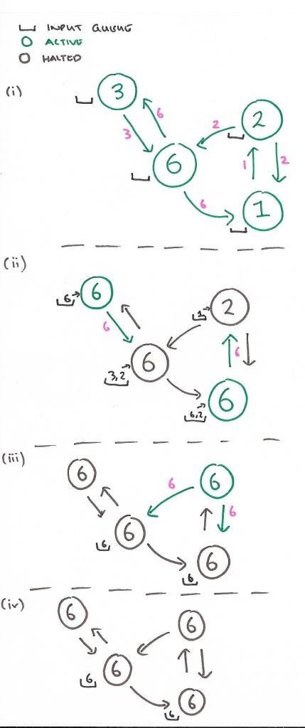
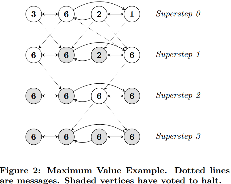
In this way there's no centralized controller, and each node is only aware of it's immediate neighbors - this allows for distributed computation and scalability across large graphs utilizing Spark and other actor frameworks like in Scala. These message passing frameworks are also inherently parallelizable, as each node can process messages and send out new messages simultaneously, which speeds up computation on large graphs

In the context of Graph Neural Networks (GNN's), message passing is used to aggregate information from neighboring nodes to update a node's representation or embedding. Each node sends its current state as a message to its neighbors, which then aggregate these messages (using functions like sum, mean, or max which are permutation invariant) to update their own states. This process is repeated for multiple iterations (or layers), allowing nodes to gather information from further away in the graph

A way to aggregate messages from neighbors is:

$$m_v^{(k)} = \text{AGGREGATE}^{(k)}(\{h_u^{(k-1)} : u \in N(v)\})$$

• Each node starts with an initial feature vector $h_v^{(0)}$ (node attributes)
• At each layer $k$, each node $v$ aggregates messages from its neighbors $N(v)$ using a permutation invariant function AGGREGATE
  • Can define this as sum, mean, max, etc or even a learnable function
• The aggregated message $m_v^{(k)}$ is then used to update the node's representation
• $m_v^{(k)}$ is the aggregated message for node $v$ at layer $k$
• $\text{AGGREGATE}^{(k)}$ is a permutation invariant function (sum, mean, max, etc)
• $h_u^{(k-1)}$ is the representation of neighbor node $u$ from the previous layer
• $N(v)$ is the set of neighbors of node $v$

In diagram below, each node aggregates messages from its neighbors (using mean aggregation) to update its own representation at each layer, and finally all of those go back to the original node after multiple layers of aggregation and transformation

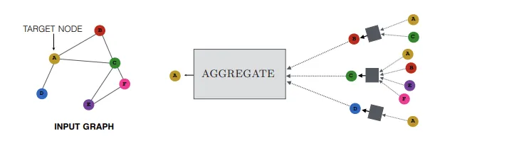
In most scenario's the AGGREGATE function is followed by a COMBINE function that merges the aggregated message with the node's own previous representation, often using a neural network layer and non-linear activation, and they mostly just need to be differentiable to allow for backpropogation

Code below shows how to implement this in Python where:

• Update and aggregate functions are nn.Linear layers followed by ReLU activations
  • Allows learnable transformations of messages and node features that may not be linearly separable
• The GNN consists of multiple layers of these message passing operations
• MessagePassing is done via matrix multiplication with the adjacency matrix to gather neighbor information
• The reason multiplying by the adjacency matrix works is that it effectively sums up the features of neighboring nodes for each node in the graph
  • If we are at node v, the row in the adjacency matrix corresponding to v has 1s for each neighbor and 0s elsewhere, and so multiplying this row by the feature matrix sums up the features of all neighbors of v (message passing!)

Show Python Code

class GNNLayer(nn.Module):
    def __init__(self, input_dim, output_dim):
        super(GNNLayer, self).__init__()
        self.update_fn = nn.Linear(input_dim, output_dim)
        self.aggregate_fn = nn.Linear(input_dim, output_dim)
    def forward(self, h, adj_matrix):
        messages = torch.matmul(adj_matrix, h)  # Aggregating messages from neighbors
        aggregated = self.aggregate_fn(messages)  # Applying the aggregate function
        updated = self.update_fn(h) + aggregated  # Updating the node embeddings
        return updated
class GNN(nn.Module):
    def __init__(self, input_dim, hidden_dim, output_dim, num_layers):
        super(GNN, self).__init__()
        self.layers = nn.ModuleList()
        self.layers.append(GNNLayer(input_dim, hidden_dim))
        for _ in range(num_layers - 2):
            self.layers.append(GNNLayer(hidden_dim, hidden_dim))
        self.layers.append(GNNLayer(hidden_dim, output_dim))
    def forward(self, features, adj_matrix):
        h = features.clone()
        for layer in self.layers:
            h = layer(h, adj_matrix)
        return h
# Example usage
input_dim = 16
hidden_dim = 32
output_dim = 8
num_layers = 3
# Generating random node features and adjacency matrix
num_nodes = 10
features = torch.randn(num_nodes, input_dim)
adj_matrix = torch.randn(num_nodes, num_nodes)
# Creating a GNN model
gnn = GNN(input_dim, hidden_dim, output_dim, num_layers)
# Forward pass through the GNN
embeddings = gnn(features, adj_matrix)
print("Node embeddings:")
print(embeddings)

Neighborhood Aggregation Methods

Neighborhood aggregation is a fundamental operation in Graph Neural Networks (GNNs) that allows nodes to gather information from their local neighborhood in the graph. The choice of aggregation method can significantly impact the performance and expressiveness of the GNN. Here are some common neighborhood aggregation methods:

• Mean Aggregation: This method computes the average of the feature vectors of a node's neighbors. It is simple and effective, ensuring that the output is invariant to the order of neighbors
  • $m_v^{(k)} = \frac{1}{|N(v)|} \sum_{u \in N(v)} h_u^{(k-1)}$
• Sum Aggregation: This method sums the feature vectors of a node's neighbors. It can capture the total influence of neighbors but may be sensitive to the number of neighbors
  • $m_v^{(k)} = \sum_{u \in N(v)} h_u^{(k-1)}$
• Max Pooling: This method takes the element-wise maximum of the feature vectors of a node's neighbors. It can capture the most prominent features among neighbors
  • $m_v^{(k)} = \max_{u \in N(v)} h_u^{(k-1)}$
• Attention Mechanism: This method assigns different weights to neighbors based on their importance, allowing the model to focus on more relevant neighbors. The weights are learned during training
  • $m_v^{(k)} = \sum_{u \in N(v)} \alpha_{vu} h_u^{(k-1)}$
  • where $\alpha_{vu}$ are attention coefficients computed using a learnable function
• LSTM-based Aggregation: This method uses a Long Short-Term Memory (LSTM) network to aggregate neighbor features, allowing for more complex interactions among neighbors
  • $m_v^{(k)} = \text{LSTM}(\{h_u^{(k-1)} : u \in N(v)\})$

Each of these methods has its own advantages and trade-offs, and the choice of aggregation method may depend on the specific application and characteristics of the graph data being used

Another important topic is how to handle nodes with varying degrees (number of neighbors) during aggregation. Techniques such as neighbor sampling (e.g., GraphSAGE) or normalization can help mitigate issues arising from high-degree nodes dominating the aggregation process.Neighbor normalization can be done by dividing the aggregated message by the degree of the node, ensuring that nodes with more neighbors do not disproportionately influence the aggregation. This is particularly important in graphs with a power-law degree distribution, where a few nodes may have a very high degree compared to others, and so we don't want them to dominate the aggregation process

Over-smoothing is just as dangerous as under-smoothing in GNNs. Over-smoothing occurs when node representations become indistinguishable after multiple layers of aggregation, leading to a loss of local information. This can happen when too many layers are stacked, causing the embeddings to converge to similar values. It essentially resolves to "everything looks the same, because we made our radius of neighbors too large" - if you look at everyone to create embeddings for everyone, they all come out to be the same. To mitigate over-smoothing, techniques such as residual connections, layer normalization, or limiting the number of layers can be employed, and implementations of these are found in libraries like PyTorch Geometric and DGL

The below script shows how to implement skip connections in a GNN layer, allowing the model to retain information from previous layers and mitigate over-smoothing. In this example, we concatenate the original node features with the aggregated messages before passing them through a linear transformation

Show Python Code with Skip Connections

class GNN(nn.Module):
    def __init__(self, input_dim, hidden_dim, output_dim):
        super(GNN, self).__init__()
        self.linear1 = nn.Linear(input_dim, hidden_dim)
        self.linear2 = nn.Linear(hidden_dim + input_dim, output_dim)
    def forward(self, h, adj_matrix):
        # Initial node representations
        h0 = self.linear1(h)
        
        # Message passing with concatenation-based skip connections
        m = torch.matmul(adj_matrix, h)
        h1 = self.linear2(torch.cat((h, m), dim=1))
        h_updated = h1 + h0  # Skip connection: add previous layer representation
        
        return h_updated

Graph Convolutional Networks

Graph Convolutional Networks (GCN's) were first introduced as a method for applying NN's to graph structured data

The simplest GCN's had three operators:

• Graph convolution
• Linear layer
• Nonlinear activation

The operations were also typically done in that order, and the Node Embedding example above showcases a similar ordering

• Aggregate local neighbors (convolution)
• Apply linear transformation (linear layer)
• Use a nonlinear $\sigma$ activation for more robust relationships

The initial workflow above inspired GraphSAGE

GraphSAGE Idea

GraphSAGE is a representation learning technique for dynamic graphs - this, in english, means that it can create node embeddings on new (previously unseen) nodes, which makes it inductive and useful for dynamic or growing graphs

The intuition is that GraphSAGE learns vector representations (embeddings) for nodes by repeatedly sampling a node's neighbors, aggregating their features (permutation invariant function), combining that with it's own features, and passing through neural layers - this is exactly what we saw above in the Node Embedding portion, and it allows generalization to new (previously unseen) nodes in the graph because it utilizes sampling and doesn't require the full adjacency matrix to compute a node's embedding. This means it doesn't require all of a node's neighbors (full adjacency matrix), and can create embeddings based on local samples

Simple Neighborhood Aggregation:

$$h_k^{(v)} = \sigma(W_k \sum_{u \in N(v)} {h_u^{(k-1)} \over {|N(v)|}} + B_k h_k^{(k-1)})$$

GraphSAGE:

$$h_k^{(v)} = \sigma([W_k \cdot \text{Agg}(\{h_u^{(k-1)} : u \in N(v)\}), B_k h_k^{(k-1)}])$$

• Generalized aggregation method: $\text{Agg}(\{h_u^{(k-1)} : u \in N(v)\})$
  • Literally just mentions any aggregation on layers before it, in it's neighborhood
  • Other options outside of typical weighted average include
    • Pooling: Transform each neighbor embedding with a NN, then apply element-wise max-pooling
      • $\text{Agg}(\{h_u^{(k-1)} \space \forall u \in N(v)\}) = \max_{u \in N(v)} \sigma(W_{\text{pool}} h_u^{(k-1)} + b_{\text{pool}})$
    • LSTM: Use a unidirectional LSTM to aggregate neighbor embeddings (requires imposing an order on neighbors, which is not inherently defined in graphs)
      • $\text{Agg}(\{h_u^{(k-1)} \space \forall u \in N(v)\}) = \text{LSTM}(\{h_u^{(k-1)} \space \forall u \in N(v)\})$
• Concatenate neighbor embedding and self embedding via the $+$ in the simple neighborhood aggregation, but you can do any other combination operation (specified as "," in the GraphSAGE equation)