Classic ML

Classic ML

A lot of this article was made for interpretability reasons, and takes from ChristophM Blog

Classic ML only became classic after LLM's came out - in reality, most LLM's are just a specific generative only, decoder only, deep learning neural network

Some neural networks are categorized as classical ML! Some deep learning models are classified as classic ML! Pretty much everything that isn't some big LLM model is getting categorized here, and it's silly

For the rest of this area / blog post classical ML will refer to regression, decision tree's, clustering, and some other area's that stay away from deep learning

Other things like Graph Neural Networks are considered "Classical ML" as well, but trying to divvy things up by concept is tough so those are placed with Graph Processing components

Linear Regression

Pretty much the "Hello, world" of ML (or maybe K-Means is) - a Linear Regression model predicts the target as a weighted sum of the feature inputs

The linearity of a learned relationship leads to many useful things, most of all interpretability

Linear models can be used to model the dependence of a regression target $y$ on features $\bold{x}$, and the learned relationshop can be written as: $\hat{y} = \beta_0 + \beta_1 x_1 + \beta_2 x_2 + ... + \beta_p x_p + \epsilon$ where the $\beta_j \in \{1, ..., p\}$ represent the learned feature weights (aka coefficients), $\beta_0$ is the intercept, and is our way to linearly shift things up, down, left, right without altering slope, and $\epsilon$ is the error that's always involved for any prediction

Errors in this sense are always assumed to follow a Gaussian distribution, and in-fact most of our input data, data variance, and pretty much any other statistical feature of linear regression can basically be assumed to have some sort of Gaussian distribution

If these assumptions hold, finding the $\beta$ coefficients can be done via gradient descent (many iterations towards finding optimal value), or directly done using analytical techniques to directly solve for them all

The actual assumptions are:

• Linearity: The regression model assumes the output target is a linear combination of features
  • If features are non-linear, then a linear regression model may not be the best fit without some tweaking
    • Tweaks may include interaction terms, regression splines, or model splits
• Normality: The target outcome given the features follows a normal distribution
  • Basically the target follows a normal distribution, given we're trying to predict it with the features we've chosen
  • If this is violated then the estimated confidence intervals of the feature weights are invalid
• Homoscedasticity: Essentially just constant variance - specifically asks the variance of the error term is assumed to be constant over the entire featur space
  • This is usually violated in practice
  • If you try to predict housing prices, the variance in errors for multi-million dollar homes will be larger than the variance for typical $500k homes
    • The variance for larger homes could be hundreds of thousands of dollars, where-as the variance for $500k typical homes may be tens of thousands
    • Errors are not based on range of predicted value, they are strictly constant
• Independence: It's assumed that each instance (features and target) are independent of any other instances
  • Repeated measurements of the same target are related data (continuously tracking home prices over time could violate this rule)
• Fixed features: The input features are fixed, meaning they're given constantss, and not statistical variables (which ultimately implies they're free of measurement errors)
• Absence of multi-collinearity: Assumes there aren't strongly correlated features - i.e. feature1 has a high correlation with feature2, because this could lead to issues estimating the weights as feature effects may no longer be additive

$\bold{\hat{\beta}} = \arg\min_{\beta_0, \ldots, \beta_p} \sum_{i=1}^n \left( y^{(i)} - \left( \beta_0 + \sum_{j=1}^p \beta_j x_j^{(i)} \right) \right)^2$

Linear Regression Interpretability

These linear equations mentioned above have an easy-to-understand interpretation at a weight level

• For numeric features: you can directly say "an increase in $x_n$ will cause a $\beta_n$ shift in the output target, all other things similar" which gives us a direct cause and effect for our input and outputs
• For binary features: The $\beta_n$ is basically all or nothing so if you do not include it, then the target doesn't deviate from the average for that feature
• For categorical variables: Typically you just one-hot-encode things, set one specific category as reference, and interpret them as reference vs other for all categories

These estimated weights, $\beta_n$, come with confidence intervals, which basically are ranges for the weight estimate that covers the "true" weight with a certain confidence. Meaning a 95% confidence interval for a weight of 2 means the true value could range from 1 - 3. The interpretation is "If you repeated the estimation 100 times with newly sampled data, the confidence interval would include the true weight 95 / 100 times, given that the linear regression model is the correct model for the data", where correctness depends on whether the relationships in data meet all of the underlying linear regression assumptions

$\bold{R^2}$ will tell us how much of the total variance of target outcome is explained by the model. 0 means if doesn't explain anything at all, and 1 means the variance is perfectly explained - if it's negative that means SSE $\gt$ SST and that a model doesn't capture the trend of data, and fits worse than using the mean of the target as a predictions: $R^2 = 1 - {{SSE} \over {SST}}$

$\bold{SSE}$ is the squared sum of the error terms, which tells us how much variance remains after fitting the linear model: $SSE = \sum_{i=1}^{n} (y^{(i)} - \hat{y}^{(i)})^2$

$\bold{SST}$ is the squared sum of data variance, which is the total variance of the target outcome: $SSE = \sum_{i=1}^{n} (y^{(i)} - \bar{y})^2$

Lastly, the importance of a feature in a linear regression model can be measured by the absolute value of it's t-statistic, which is the estimated weight scaled with its standard error. The importance of a feature increases with increasing weight, i.e. the more variace the estimated weight has (the less certain you are about it), the less "important" the feature is: $\bold{t_{\hat{\beta}_j}} = \hat{{\beta}_j \over {SE({\beta}_j)} }$

Sparse Linear Models

What if you have models with hundreds of thousands of features? Interpretability goes downhill, and ultimately our model becomes a jumbled mess of data. In scenarios like this you can introduce sparsity (= a few features) into linear models directly

Lasso

Lasso is an automatic way to introduce sparsity into linear regression models - Lasso stands for "Least Absolute Shrinkage and Selection Operation" and so when it's applied to a linear regression model it will perform feature selection and regularization of selected feature weights

In typical linear regression, our weights look to solve: $\min_{\beta}({1 \over n} \sum_{i=1}^n (y^{(i)} - \bold{x}^{(i)T} \bold{\beta})^2)$

In Lasso you add a new term: $\min_{\beta}({1 \over n} \sum_{i=1}^n (y^{(i)} - \bold{x}^{(i)T} \bold{\beta})^2 + \lambda||\bold{\beta}||_1)$

Where $||\bold{\beta}||_1$ is the L1-norm of the feature vector, which will ultimately penalize large weights. Since L1 is used, most of the weights receive an estimate of 0, and others are shrunk. $\lambda$ is the regularization parameter and is manually tweaked with cross-validation data - the larger the $\lambda$ the more weights become 0.

Logistic Regression

Logistic regression models the probabilities for classification problems with two possible outcomes - it's essentially an extension of linear regression model for class outcomes

Why Cant you Use Linear

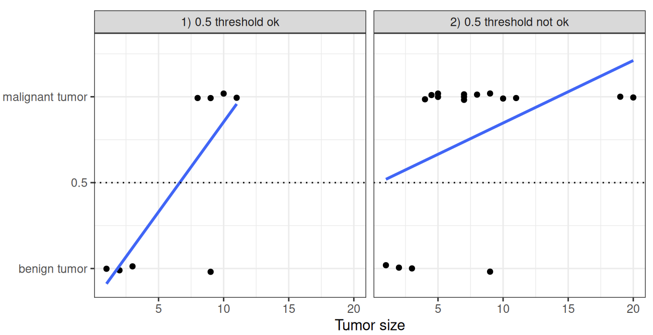
Why can't you just use linear regression for classification? In the case of two classes, 0 or 1, a linear model doesn't output probabilities, but it treats the classes as numbers (0 and 1) and fits the best hyperplane that minimizes the distances between the points and the hyperplane. In laymen terms, it simply interpolates between the points, and it's not able to be interpreted as probabilities - i.e. the interpretation of the model would be incorrect. There's no meaningful threshold to use as one or the other, and the problems become even worse with multiple classes - the higher the value of a feature with a positive weight, the more it contributes to the prediction of a class with a higher number, even if classes that heppen to get a similar number are no closer than the first and last classes.

Logistic Theory

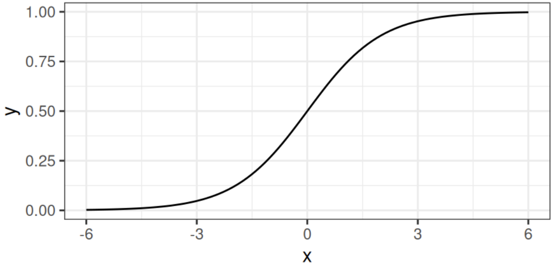
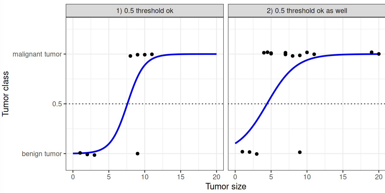
A solution for classification is therefore logistic regression. Instead of fitting a straight line or hyperplane, the logistic regression model uses the logistic function to squeze the output of the linear equation between 0 and 1

$\text{logistic}(\bold{z}) = { 1 \over {1 + \text{exp}(-\bold{z})}}$

In Linear Regression you have: $y = \beta_0 + \beta_1 x_1 + \beta_2 x_2 + ... + \beta_p x_p + \epsilon$

In Logistic Regression you have: $P(Y^{(i)} = 1) = \text{logistic}(\bold{x}^{(i)T}\bold{\beta}) = {1 \over {1 + \text{exp}(-(\beta_0 + \beta_1 x_1 + \beta_2 x_2 + ... + \beta_p x_p))}}$

The main difference above is you take the linear portion and insert it into an exponential function - if you decode the equation you get:

• If $\text{exp}(-(\beta_0 + \beta_1 x_1 + \beta_2 x_2 + ... + \beta_p x_p))$ comes out to be 0, then our logistic model is $1 \over 1$
  • Therefore, the smaller the $\text{exp}(...)$ portion is, the closer our model is to 1
• The $\text{exp}(...)$ portion is
  • 0 if
  • higher if

This difference brings the tumor example above to:

Interpretation

Interpreting logistic regression is a bit weirder since the outcome in logistic regression is a probability between 0 and 1 - the weights no longer influence the probability in a linear fashion

To interpret the weights the equation needs to be re-formulated so that the $\beta_0 + \beta_1 x_1 + \beta_2 x_2 + ... + \beta_p x_p$ is on the right side of the equation by itself

$\ln({P(Y = 1) \over 1 - P(Y = 1}) = \ln({P(Y = 1) \over P(Y = 0}) = \beta_0 + \beta_1 x_1 + \beta_2 x_2 + ... + \beta_p x_p$

$\ln({P(Y = 1) \over P(Y = 0})$ is known as the odds which is the probability of an event divided by probability of no event and wrappd in a logarithm, therefore called "log odds"

Altogether logistic regression is a linear model for the log odds, if you interpret the log odds as our output $\hat{y}$

${P(Y = 1) \over 1 - P(Y = 1} = \text{odds} = \text{exp}(\beta_0 + \beta_1 x_1 + \beta_2 x_2 + ... + \beta_p x_p)$

**no negative

${\text{odds}_{x_{j}+1} \over \text{odds}_{x_{j}}} = {\text{exp}(\beta_0 + \beta_1 x_1 + \beta_2 x_2 + ... + \bold{\beta_{j} x_{j}+1} ... + \beta_p x_p) \over \text{exp}(\beta_0 + \beta_1 x_1 + \beta_2 x_2 + ... + \bold{\beta_j x_j} ... + \beta_p x_p)}$

Then, you can cancel a bunch of crap because ${\text{exp}(A) \over \text{exp}(B)} = \text{exp}(A-B)$

Sooooo ${\text{odds}_{x_{j}+1} \over \text{odds}_{x_{j}}} = \text{exp}(\beta_{j} (x_{j}+1) - \beta_{j} x_{j}) = \text{exp}(\beta_{j})$

So in the end $\text{exp}(\beta_{j})$ is the feature weight for a specific $x_j$, an so a change by one unit changes the odds ratio (multiplicative) by a ratio of $\text{exp}(\beta_{j})$

Therefore, the interpretation comes out to "A change in $x_{j}^{(i)}$ (i.e. the ith row's $x_j$ value) by one unit increases the log odds ratio by the value of the corresponding weight"

Interpreting the log odds is weird too - for example if you have odds of 2 it means $P(Y=1)$ is twice as high as $P(Y=0)$ so having a weight of 0.7 would then increase the log odds ratio by $\text{exp}(0.7) \approx 2$ and the resulting log odds would be $\approx$ 4. Usually no one deals with the odds and people just interpret the weights as the odds ratio's instead, because to calculate actual odds you need to set a value for each feature, which would then only make sense if you want to look at one specific instance of a dataset (most people look at all instances).

After that, the rest of the interpretation is the same as Linear Regression:

• For numerical features: If you increase the value of $x_{j}^{(i)}$ by one unit, the estimated odds change by a factor of $\text{exp}(\beta_{j})$
• For binary categorical features: One of two values of the feature is the reference category (mean / "typical value"), and so changing $x_{j}^{(i)}$ from the reference to the other category changes the esimated odds by a factor of $\text{exp}(\beta_{j})$
• For categorical features with many values: Typically you just one-hot-encode things, set one specific category as reference, and interpret them as reference vs other for all categories

GLM and GAM

Linear regression assumptions are typically violated in practice, and so Generalized Linear Models and Generalized Additive Models were created to help solve some of the issues stemming from data that doesn't fit into Linear Regression's reqiurements

Linear regression assumes the prediction of an instance can be expressed by a weighted sum of it's $p$ features with a random variable $\epsilon^{(i)}$ which follows a Gaussian distribution.

Issues With Linear Regression

• Wanting our predictions to only be positive, which cannot happen under Gaussian constraints which have 1/2 above and 1/2 below zero
  • How many minutes will this car ride be
  • How much food to eat in a day
• Most data we scrape / collect ends up being correlated or interacting in some way
• The true relationship between features and target $\hat{Y}$ is not completely and totally linear

These are common scenario's that Linear Regression models cannot overcome, and they're typical enough scenario's that most people do want to end up modeling

In this case, need something a bit more robust

GLM - Non Gaussian Outcomes

Linear regression assumes the outcome given a feature follows a Gaussian distribution, which excludes many cases such as:

• Positive only
• Categorical
• Count
• Highly skewed events (housing prices)

Generalized Linear Models are an extension of Linear Regression models that are stood up to specifically tackle this issue

The core idea is Keep the weighted sum of the features, but allow non-Gaussian outcome distributions and connect the expected mean of this distribution and the weighted sum through a non-linear function

Basically, this means keep the weighted sum setup, but tie this weighted sum to an expected mean in a non-gaussian distribution by using some new function

Old LR formula: $\hat{y} = \beta_0 + \beta_1 x_1 + \beta_2 x_2 + ... + \beta_p x_p + \epsilon$

A potential GLM formula: $\hat{y} = g(\beta_0 + \beta_1 x_1 + \beta_2 x_2 + ... + \beta_p x_p) + \epsilon$

Where $g(\cdot)$ is a non-linear function that helps to map our linear output to a non-gaussian distribution

Logistic Regression is actually an example of this where the model assumes a Bernoulli Distribution for the outcome variable and links the expected mean of that Bernoulli Distribution and the weighted sum of $\beta_j x_j$ using the logistic function - meaning $g(\cdot)$ is the logistic function

Formally, the equation is $g(E[Y | \bold{x}]) = \beta_0 + \beta_1 x_1 + \beta_2 x_2 + ... + \beta_p x_p = \bold{x}^T \beta$

The above equation equates to "the link function connects the expected value of the outcome (possibly transformed) to the linear predictors" - outcome is modeled using a probability distribution from exponential family

And GLM's consist of 3 components:

• Link function $g(\cdot)$
• The weighted sum $\bold{x}^T \beta$
• Probability distribution from the exponential family that defines $E_Y$
  • This exponential family is a set of distributions that can be written with the same formula (it has parameters to "tweak" it to map to new formulas) that includes an exponent, mean, and variance of a distribution
  • Essentially the exponential family is a parameterized distribution setup that allows us to create distributions with certain profiles using parameters
  • There are a lot - Wikipedia List of Exponential Family

Any exponential distribution from that family can be used for a GLM, and they are chosen based on what you'd like to predict:

• Outputting a count typically uses the Poisson Distribution
  • Natural logarithm as link function and Poisson as expected distribution allow us to model things like "number of coffee's drank in a day"
• Positive only events typically use the Exponential Distribution
• Probabilities and odds are tpyically done using Bernoulli Distribution
  • Logistic function is the link function
• etc...

Each exponential family distribution has a canonical link function that can be derived mathematically from the distribution - so how do you choose the right distribution and link function? There's no perfect recipe... Typically, you just choose functions that respect the domain of the expected distribution / problem. A good recipe is to try and use a link function / distribution that resembles the data gathering process, but it's not always easy to tell what this process is! Plotting the data can showcase it at times.

Our classic Linear Regression model can also be modeled this way, but $g(\cdot)$ is just the identity function

GLM Interpretation