Numerical Computation and Optimization

Numerical Computation

Most of the algo's discussed in courses are general that should work in theory, but making them actually work on a computer is difficult - numerical computation is all around how to get things to run efficiently on a computer, and what's typically done in industry

A good example is linear regression - a fair amount of theory is around interpreting the coefficients and understanding the model, but when it comes to actually implementing it, there are many practical considerations such as numerical stability, convergence, and optimization techniques that need to be taken into account to solve it analytically for billions of examples (also none of the underlying assumptions ever hold in real life)

Trying to shove a billion row and hundred of thousand feature matrix into a single machine to solve linear regression is a recipe for disaster. Instead, techniques like mini-batch gradient descent, distributed computing, and specialized hardware (like GPUs) are often employed to make the problem tractable

To make things even worse most real numbers on machines only have a finite precision representation (e.g., float32, float64), which can lead to some instability, but then multiplying these small numbers can quickly lead to underflow or overflow issues, vanishing or exploding gradients, and other numeric issues that can arsise during optimization, training, and inference

Overflow and Underflow

Overflow and underflow are two common issues that can arise during numerical computation, particularly when dealing with floating-point numbers. We can't represent an infinite number of real numbers with a finite number of bits, so there are approximation errors for almost all real numbers - this is compounded as there are more arithmetic operations performed, especially multiplication and division

• Overflow occurs when a calculation produces a result that is larger than the maximum representable value for a given data type. For example, if you try to compute the exponential of a large number (e.g., $e^{1000}$), the result probably exceeds the maximum value that can be represented by a float64, leading to an overflow error
• Underflow, on the other hand, happens when a calculation produces a result that is smaller than the minimum representable value (but not zero) which get rounded down to 0. One particular pitfall is division by 0, instead of a small real number. This often occurs when dealing with very small numbers, such as probabilities. For instance, if you multiply a series of small probabilities together, the result may become so small that it is rounded down to zero, leading to underflow
  • Just taking the inverse, $1 \over {e^{1000}}$ can lead to underflow

Representing a number that's over or under flowed can lead to inf, NaN, or 0 values in computations, which can propagate through calculations and lead to incorrect results or failures in algorithms which then require careful debugging to figure out where an approximation on a random Tuesday occurred

It's a fairly straightforward problem here, but in practice these issues can lead to significant inaccuracies in computations, especially in iterative algorithms like gradient descent where small errors can accumulate over time. In gradient descent you're multiplying small learning rates with small gradients, which can lead to underflow if not handled properly, and adding large gradients across thousands of iterations can lead to overflow

A common example is the Softmax Function which is used to predict probabilities associated with a multinoulli distribution. The softmax function involves exponentiating the input values, which can lead to overflow for large input values. To mitigate this, a common technique is to subtract the maximum input value from all input values,$\bold{z} = \bold{x} - \max_i(\bold{x}_i)$, before applying the softmax function. This helps to keep the exponentiated values within a manageable range and prevents overflow, while also preserving the relative differences between the input values

• This brings the largest item to 0, which removes the risk of overflow when exponentiating, since $e^0 = 1$ is the largest value now
• This also ensures at least one term in the denominator is 1, preventing division by zero
• Underflow is still an issue for Softmax, specifically when all input values are very negative and running $\log$ on the output probabilities - this can be mitigated by using the log-sum-exp trick, which is a numerically stable way to compute the logarithm of a sum of exponentials

The above is one example of an extremely common function, and pretty much each function in a low-level library has to deal with these numerical stability issues in some way, but common folk don't necessarily have to worry about it when using high-level libraries like TensorFlow or PyTorch since these libraries have already implemented these stability techniques under the hood

Poor Conditioning

Conditioning refers to how sensitive a function or algorithm is to small changes in its input. In numerical computation, poor conditioning can lead to significant errors in the output, even when the input changes only slightly. This is particularly problematic in optimization algorithms, where small perturbations in the input can lead to large changes in the output, making it difficult to converge to a solution

Obviously numerical precision plays a big role here, as small changes to an approximation of a real number can lead to drastically different results, so that it seems almost non-deterministic when running the same algorithm multiple times with slightly different initial conditions or random seeds

The function $f(\bold{x}) = \bold{A}^-1 \bold{x}$, where $\bold{A}^-1 \in \mathbb{R}^{n \times n}$ is a matrix. If it has an eigenvalue decomposition it's condition number is defined as the ratio of the largest eigenvalue to the smallest eigenvalue, $\kappa(\bold{A}) = {|\lambda_{max}| \over |\lambda_{min}|}$. If the condition number is large, it indicates that the function is poorly conditioned, meaning that small changes in the input can lead to large changes in the output. The sensitivity is a property of the matrix itself, and not rounding errors or numerical precision - it's something you simply have to deal with.

The inverse function applied to inputs, $\bold{A}^-1 \bold{x}$, is a fairly used operation throughout numerical computation, and if $\bold{A}$ is poorly conditioned, then small changes in $\bold{x}$ can lead to large changes in the output. This can make it difficult to solve systems of linear equations or perform other operations that involve matrix inversion

Gradient Based Optimization

Most ML / DL algorithms involve optimizations, and most of them involve gradient descent or some variant of it

Optimization in this sense means minimizing or maximizing some objective function $f(\bold{x})$ with respect to its parameters $\bold{x}$ - this objective function is also known as cost function, loss function, energy function, or error function depending on the context, but they all refer to the same thing - a function that quantifies how well a model is performing, and the goal of optimization is to find the parameters that minimize (or maximize) this function

The value that minimizes or maximizes this function is known as the Optimum and is referred to as $\bold{x}^*$ with a $*$ superscript

$\bold{x}^* = \arg \min_{\bold{x}} f(\bold{x})$

Gradient descent is an iterative optimization algorithm used to minimize a function by iteratively moving in the direction of steepest descent, as defined by the negative of the gradient. So of course in practice as you're moving around numbers typically between $[-1, 1]$ with small learning rates (e.g., $0.001$), you can easily run into underflow issues where the updates become so small that they get rounded down to zero, effectively halting the optimization process - this is known as the Vanishing Gradient problem

Quick Calculus Review

For a specific function $y = f(x)$ where both $x$ and $y$ are real numbers, the derivative $f'(x)$ represents the rate of change of $y$ with respect to $x$. In the context of optimization, the gradient (or derivative) is used to determine the direction in which to update the parameters in order to minimize the objective function

The rate of change of $y$ with respect to $x$ essentially tells us how much a one unit change in $x$ will affect the value of $y$

The derivative $f'(x)$ is a fundamental concept in calculus and is defined as the limit of the average rate of change of the function over an interval as the interval approaches zero:

$f'(x) = \lim_{\Delta x \to 0} \frac{f(x + \Delta x) - f(x)}{\Delta x}$

In practice, the derivative gives the slope of $f(x)$ at the point $x$, and specifically is defined around an $\epsilon$-neighborhood of $x$ - $f(x + \epsilon) \approx f(x) + \epsilon \cdot f'(x)$ for small $\epsilon$

So how does this help us? The derivative helps us to minimize a function by telling us how to alter $x$ to make a small improvement in some direction for $y$ - meaning if our $y$ is "wrong" in some direction, we can move it more towards the "right" direction by altering $x$ in some way, and we can mathematically figure this out using the derivative

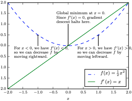
Where the slope is 0, we know there's a min or max, and using a second-order derivative test can help us determine which one it is. The second derivative $f''(x)$ tells us about the curvature of the function at that point: if $f''(x) > 0$, we have a local minimum, and if $f''(x) < 0$, we have a local maximum

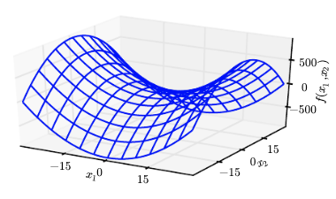
Global min / max is determined by evaluating the function at critical points and endpoints, and comparing their values to find the absolute minimum or maximum over the entire domain, but in practice gradient descent can converge to a local minimum rather than the global minimum, especially in non-convex optimization problems - below, we'd just tweak $x$ a bit to get closer to the bottom of the valley

$f(x + \epsilon) \approx f(x) + \epsilon \cdot f'(x)$

To

$f(x - \epsilon \cdot \text{sign}(f'(x))) \approx f(x) - \epsilon \cdot (f'(x))^2$

The $sign(f'(x))$ function returns $1$ if the derivative is positive, $-1$ if it's negative, and $0$ if it's zero. This means that if the derivative is positive, we subtract a small value from $x$ to decrease $f(x)$, and if the derivative is negative, we add a small value to $x$ to also decrease $f(x)$

We know $f(x - \epsilon \cdot \text{sign}(f'(x)))$ is less than $f(x)$ since $(f'(x))^2$ is always non-negative, so by updating $x$ in the direction opposite to the sign of the derivative, we can decrease the value of the function - if we reduce $f(x)$, we are reducing $y$

This all then happens multi-dimensionally, and so instead of computing the derivative with respect to a single $x$ input, we must compute the partial derivative with respect to each input dimension $x_i$ in the input vector $\bold{x}$ for $y$ - the partial derivative $\frac{\partial f}{\partial x_i}$ represents the rate of change of $f$ with respect to $x_i$, while keeping all other input dimensions constant

The Gradient is actually defined as the vector of all partial derivatives with respect to each input dimension, denoted $\nabla_x f(\bold{x})$ or $\bold{grad} f(\bold{x})$, and critical points occur where the gradient is zero, meaning all partial derivatives are zero simultaneously

The directional derivative in the direction $\bold{u}$ is the slope of the function $f$ in the direction of $\textit{u}$

This directional derivative is equivalent to $f(\bold{x} + \alpha \cdot \bold{u}) \approx f(\bold{x}) + \alpha \cdot \nabla_x f(\bold{x}) \cdot \bold{u}$ evaluated at $\alpha = 0$

From this, and the chain rule, the derivative will equate to $\frac{\partial f(\bold{x} + \alpha \cdot \bold{u})}{\partial \alpha}$

Which simplifies to the directional vector multiplied by the gradient $\bold{u}^{T} \nabla_x f(\bold{x})$

Therefore, to minimize $f$ we would like to find the direction in which $f$ decreases the fastest which is given by the negative gradient $-\nabla_x f(\bold{x})$ - why? $\min_{\bold{u}} \bold{u}^{T} \nabla_x f(\bold{x})$

Equates to $\min_{\bold{u}} ||\bold{u}|| \cdot ||\nabla_x f(\bold{x})|| \cdot \cos(\theta)$

Where $\theta$ is the angle between $\bold{u}$ and $\nabla_x f(\bold{x})$. Most proofs will put ||u||$$ as a unit vector to make things easy, so it simplifies to 1$

This ends up equating to $\min_{\bold{u}} \cos(\theta)$

This is minimized when $\cos(\theta)$ is at its minimum value, which is $-1$, which occurs when $\bold{u}$ points in the opposite direction of the gradient $\nabla_x f(\bold{x})$.

Therefore, the gradient points uphill (the direction of steepest ascent), and the negative gradient points downhill (the direction of steepest descent). This is why, in gradient descent algorithms, we update our parameters in the direction of the negative gradient to minimize the objective function

$\bold{x}^{`} = \bold{x} - \eta \cdot \nabla_x f(\bold{x})$

Where $\eta$ is the learning rate, which controls the step size of each update - how do you choose this rate?

• Constant rate: If it's too large you could overshoot the minimum, and if it's too small the convergence will be slow
• Adaptive rate:
  • Line Search: Evaluating $f(\bold{x} - \epsilon \cdot \nabla_x f(\bold{x}))$ for different $\epsilon$ values to find the optimal step size at each iteration
    • This is a highly computationally expensive approach since it requires multiple evaluations of the objective function per iteration
  • Backtracking Line Search: A more efficient approach that starts with a large step size and reduces it until a sufficient decrease in the objective function is observed
  • Adaptive Methods: Techniques like AdaGrad, RMSProp, and Adam adjust the learning rate based on the history of gradients, allowing for more efficient convergence

Jacobian and Hessian

Jacobian and Hessian are just extensions of Gradients that work on partial derivatives and store results in a vector

They make doing gradient optimizations more efficient by using matrix multiplication and vector multiplication

They're useful for storing all of the partial derivatives of a function whose inputs and outputs are both vectors

The Jacobian is the matrix of all first-order partial derivatives of a vector-valued function, while the Hessian is the matrix of all second-order partial derivatives

For a function $f: \mathbb{R}^m \rightarrow \mathbb{R}^n$, the Jacobian is an $n \times m$ matrix, while the Hessian is an $n \times n$ matrix

$J_{i, j} = \frac{\partial \bold{f}(\bold{x})_{i{}}}{\partial x_j} : \bold{J} \in \mathbb{R}^{n \times m}$

$H_{i, j} = \frac{\partial^2 f(\bold{x})}{\partial x_i \partial x_j} : \bold{H} \in \mathbb{R}^{n \times n}$

The Hessian is a symmetric matrix as long as the second partial derivatives are continuous, the partial of $i$ applied to $j$ is the same as $j$ applied to $i$ as long as things are well defined

Therefore, the Hessian is real and symmetric - so we're able to decompose it into a set of real eigenvalues and an orthogonal basis of eigenvectors. The second derivative in a specific direction is represented by a unit vector $\bold{d}$ given by $\bold{d}^{T} \bold{H} \bold{d}$. The corresponding eigenvalue is the amount of curvature in that direction. The maximum eigenvalue determines the maximum second derivative (i.e. the maximum curvature)

This is helpful, as the maximum eigenvalue gives us the direction we can expect a gradient descent step to perform

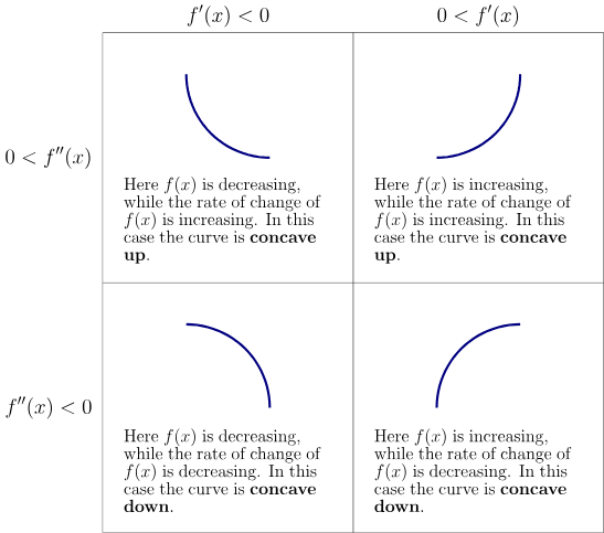
So as before, first derivative tells us the direction of steepest ascent, while the second derivative tells us about the curvature of the function in that direction

How do we interpret curvature? Suppose there's a quadratic function (or a function that locally behaves as a quadratic function)

• If the second derivative of this function is $0$, then there's no curvature and it's a perfectly straight line. At this point it's value can be perfectly predicted using the gradient - if the gradient is $1$, then a step size of $\eta$ will result in a new value of $1 + \eta$
• If the second derivative is negative, the function curves downwards, so the cost function would actually decrease more than $\eta$ (like a ball accelerating downhill)
• Same thing for positive - it would actually decrease by less than $\eta$ (like a ball decelerating uphill)

Therefore, the Jacobian helps us to find the multi-dimensional steepest ascent direction, while the Hessian provides information about the curvature in that direction

Taylor Series

Instead of computing the Hessian directly, we can use a Taylor series expansion to approximate the function around a point. The second-order Taylor series expansion of a function $f(\bold{x})$ around a point $\bold{x}_0$ is given by:

$f(\bold{x}) \approx f(\bold{x}_0) + \nabla f(\bold{x}_0)^T (\bold{x} - \bold{x}_0) + \frac{1}{2} (\bold{x} - \bold{x}_0)^T \bold{H} (\bold{x} - \bold{x}_0)$

Where $\nabla f(\bold{x}_0)$ is the gradient at $\bold{x}_0$ and $\bold{H}$ is the Hessian matrix at $\bold{x}_0$

With a learning rate of $\eta$, we can use this Taylor series expansion to perform a gradient descent step:

$\bold{x}_{1} = \bold{x}_{0} - \eta \bold{g}$

Which we can substitute to obtain

$f(\bold{x}_{0} - \eta \bold{g}) \approx f(\bold{x}_{0}) - \eta \bold{g}^T \bold{g} - \frac{\eta^2}{2} \bold{g}^T \bold{H} \bold{g}$

Which has 3 major portions:

• The original value of the function
• The expected improvement due to the slope of the function, i.e. the linear approximation (first-order term)
• The correction we apply to account for the curvature, i.e. the quadratic approximation (second-order term)
  • If this part is too large we can actually move back uphill (go into the valley and back up)
  • If $\bold{g}^T \bold{H} \bold{g}$ is too large the taylor series can predict increasing $\eta$ forever will decrease $f$ forever

Altogether, this taylor series expansion helps to compute this gradient, and reduces overall complexity into a localized area, but it can start to degrade with a large enough $\eta$

So how to choose $\eta$ heuristically?

• Line search and other computationally expensive steps are mentioned above
• Theoretically, it mostly revolves around utilizing first and second derivative tests - however, since most of the time it's a multi-dimensional optimization problem there's a need to consider the Jacobian and Hessian

The eigendecomposition of the Hessian matrix can provide info on curvature of multi-dimensional space such as local max, min, or saddle point. As we view the eigenvalues, they can provide following info:

• All positive = local min
• All negative = local max
• Mixed = saddle point
  • 

The condition number of the Hessian (ratio of smallest over largest) can also provide info on the sensitivity of the optimization problem to changes in the input space. A high condition number indicates that the problem is ill-conditioned, meaning that small changes in the input can lead to large changes in the output

Optimization Problems

Taking a look at Newton's method - it is an iterative optimization algorithm that uses the first and second derivatives of a function to find its local maxima and minima. The update rule for Newton's method is given by:

$\bold{x}_{1} = \bold{x}_{0} - \eta \bold{H}^{-1} \nabla f(\bold{x}_{0})$

Where $\bold{H}$ is the Hessian matrix at $\bold{x}_{0}$ and $\nabla f(\bold{x}_{0})$ is the gradient at $\bold{x}_{0}$. This update rule incorporates both the gradient and the curvature information provided by the Hessian, allowing for more informed steps towards the optimum, but it's referred to as the "simplest" because it assumes that the Hessian is constant over the optimization step

Near saddle points, the behavior of Newton's method can be problematic. Since the Hessian may have both positive and negative eigenvalues, the update step can lead to large changes in the optimization variable, potentially causing divergence or oscillations. In such cases, modifications to the basic Newton's method, such as adding a damping factor or using a trust region approach, may be necessary to ensure convergence

Optimization algorithms that use only the gradient, such as gradient descent, are known as First Order Optimization Algorithms

Optimization algorithms that also use the Hessian, such as Newton's Method, are known as Second Order Optimization Algorithms

In practice, most ML and Deep Learning algorithms tend to design optimization algorithms for limited families of functions, meaning there's no perfect one-size fits all solution

We can gain some guarantee's (one size fits all) if we restrict attention to functions that have certain properties, such as:

• Convexity: If the function is convex, any local minimum is also a global minimum, making optimization easier
  • Means the Hessian is positive semi-definite everywhere
  • I.e. they lack saddle points
• Smoothness: If the function is smooth (i.e., has continuous derivatives), optimization algorithms can make more informed steps
• Lipschitz Continuity: If the function satisfies a Lipschitz condition, we can bound the optimization error and ensure convergence
  • Lipschitz continuity implies that the function does not change too rapidly, which helps in ensuring that optimization steps are stable and converge to a solution
  • The below constraint basically says "don't let the gradients change too quickly"
  • It is defined via a Lipschitz constant $L$, which satisfies: $\forall\bold{x}, \forall\bold{y}, \|\nabla f(\bold{x}) - \nabla f(\bold{y})\| \leq L \|\bold{x} - \bold{y}\|$

Lipschitz continuity is a weaker constraint, but convex optimization is a much stricter constraint that requires the function to be both Lipschitz continuous and convex

Constrained Optimization

Constrained optimization refers to maximizing or minimizing an objective function inside some set $\bold{S}$ instead of the entire potential metric space

$\bold{x} \in S$ are known as feasible points, and the set of all feasible points is known as the feasible set

In terms of gradient descent, this usually means checking around some $\epsilon$-neighborhood of the current point to see if any of those points are in the feasible set, and then picking the one that results in the largest decrease in the objective function. We can do this in multiple different ways:

• Can simply restrict ourselves into that neighborhood
  • In line search for example, we can check only points that are in the feasible set
• Can project the point back into the feasible set after each update
  • For example, if we have a constraint that all elements of $\bold{x}$ must be non-negative, after each gradient descent update, we can set any negative elements of $\bold{x}$ to zero
• Can use Lagrange multipliers to incorporate the constraints into the objective function
  • This involves adding a term to the objective function that penalizes violations of the constraints, allowing us to optimize the modified objective function without explicitly checking the constraints at each step

Talking more about the Lagrange example - the idea is to design a different, unconstrained optimization problem whose solution can be converted into a solution for the original

A quick example is trying to minimize $f(x) \forall x \in \mathbb{R}^2$ constrained to $x$ having $L^2$ norm less than or equal to 1. Instead of directly solving that, we can instead minimize $g(\theta) = f([cos\theta, sin \theta]^T)$ with respect to $\theta$, and then return $x^* = [cos\theta^*, sin \theta^*]^T$ as the solution to the original problem

Finding the transformation above in practice requires creative thinking, but there's a more generalized approach using Lagrange multipliers

In doing so, we must first describe $S$ in terms of $m$ functions $g^{(i)}$ and $n$ functions $h^{(j)}$ which are known as equality constraints and inequality constraints respectively. At that point $S = \{\bold{x} | \forall i, g^{(i)}(\bold{x}) = 0; \forall j, h^{(j)}(\bold{x}) \leq 0 \}$

Suppose we want to minimize a function $f(\bold{x})$ subject to an equality constraint $g(\bold{x}) = 0$. We can introduce a Lagrange multipliers $\lambda$ and $\alpha$ and define the Lagrangian function: $= f(\bold{x}) + \sum_{i} \lambda_i g^{(i)}(\bold{x}) + \sum_{j} \alpha_j h^{(j)}(\bold{x})$

The intuition here is that we can solve a constrained optimization problem using unconstrained optimization techniques, and as long as at least one feasible point exists, and $f(\bold{x})$ is not permitted to have value $\infty$, we can find a solution

Moreover, the below equalities have the same optimal objective function values and set of optimal points $\bold{x}$

$min_{\bold{x}} max_{\lambda} max_{\alpha, \alpha \geq 0} \mathcal{L}(\bold{x}, \lambda, \alpha)$ $min_{\bold{x}} f(\bold{x})$

Why? Because any time the constraints are satisfied we have

$max_{\lambda} max_{\alpha, \alpha \geq 0} \mathcal{L}(\bold{x}, \lambda, \alpha) = f(\bold{x})$

And any time the constraints are violated, it's equal to $\infty$

To find the optimal solution, we take the gradients of the Lagrangian with respect to both $\bold{x}$ and $\lambda$, and set them to zero: $\nabla_{\bold{x}} \mathcal{L}(\bold{x}, \lambda, \alpha) = \nabla f(\bold{x}) + \lambda \nabla g(\bold{x}) + \alpha \nabla h(\bold{x}) = 0$ $\frac{\partial \mathcal{L}(\bold{x}, \lambda, \alpha)}{\partial \lambda} = g(\bold{x}) = 0$

Lagrange Intuition

The above never really sat well with me - it doesn't explain why it intuitively matters or helps anyone

Let's set it up - Given $g(x, y) = c$, we want to maximize $f(x, y)$

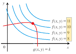
Ideally, we can just set $f'(x, y) = 0$ and use some basic calculus to find the max! It'd be wonderful. But this doesn't take the constraint into account

So what mathematical setup can be produced so there's a way to maximize that function while also taking the constraint into account? The Lagrange Multipliers are specifically designed to do that!

Rewrite $g$: $g(x, y) = c \therefore g(x, y) - c = 0$

$0 \times constant = 0$: $\lambda \times (g(x, y) - c) = 0$

Adding $0$ to anything is simply that value: $f(x, y) = f(x, y) + \lambda \times (g(x, y) - c)$

At this point we're fairly close - there's a function that's equal to our original function, but it takes our constraint into account

The partial derivative of this new function with respect to $\lambda$ is would give us intuition on how our function $f$ changes as our multiplier changes $\frac{\partial L}{\partial \lambda} = g(x, y) - c = 0$

It also equates out to $g(x, y) - c$, which we know is equal to $0$ - this means as long as this partial derivative is equal to $0$, we are satisfying our constraint!

What can we do with this? We can use it to find the optimal values of $x$ and $y$ that maximize our function while satisfying the constraint. We will use gradients, as they take all partial derivatives into a vector, and we will set the gradient of our Lagrangian to zero: $\nabla_{\bold{x}} \mathcal{L}(\bold{x}, \lambda, \alpha) = 0 = \nabla f(\bold{x}) + \lambda \nabla g(\bold{x})$

As we set this gradient to $0$ and solve for it, we guarantee that the constraint is met and that we solve for the optimal values of $x$ and $y$!

Next would be if the constraint is $g(x, y) < c$ where there's some constraint region instead of a strict line - in this scenario most of the above still holds, except our Lagrangian will need to account for the inequality constraint. This is typically done by introducing a slack variable $s \geq 0$ such that $g(x, y) + s^2 = c$

As long as $s^2$ is non-zero, there's bound to be a feasible solution that satisfies the constraint:

• $s$ is non-zero
• Therefore, $g(x, y) - c < 0$

$g(x, y) < c \rarr g(x, y) - c < 0$

$s$ is known as the slack variable

The Lagrangian is then defined as: $\mathcal{L}(x, y, \lambda, s) = f(x, y) + \lambda (g(x, y) + s^2 - c)$

Example: Linear Least Squares