Linear Algebra Notes
Linear Algebra
All of the old notes I have on Linear Algebra topics, plus 3Blue1Brown, and some DL Books
Combining this with the Probability and Statistics section is basically ML and Effects Testing
Definitions
- Scalar: A single number, often representing a quantity in space
- Often written in italics, e.g., .
- Vector: An ordered array of numbers, which can represent a point in space, or direction in physics, where each element gives the coordinates along a different axis
- Often written in bold, e.g.,
- Can identify each individual number by it's index - i.e.
- A vector having elements would have
- Can subset a vector
- for contiguous subset
- for a defined index set
- for all numbers except number at index 1
- Norm: A measure of the length (magnitude) of a vector. Intuitively they measure how far a vector is from the origin (or point we are measuring from)
- Norms map vectors to non-negative numbers
- Commonly used norms:
- Norm (Manhattan Norm):
- Norm (Euclidean Norm):
- Extremely common in ML - it's mostly noted as without the subscript
- Squared Norm can be calculated easily via the Dot Product:
- Formally,
- Commonly used to measure distances between points in space, or to regularize models in machine learning to prevent overfitting
- Matrix: A 2-D array of numbers, which can also represent a linear transformation, or a system of linear equations
- Often written in italic uppercase bold, e.g.,
- A matrix having rows and columns would have
- Can identify each individual element by its row and column indices - i.e.
- Can identify an entire row - i.e.
- Or an entire column - i.e.
- Tensors: A generalization of scalars, vectors, and matrices to higher dimension. They can also be defined as an array with more than 2 axes. "An array of numbers arranged on a regular grid with a variable number of axes (dimensions) is known as a tensor"
- Tensors are denoted by boldface type, e.g.,
- To access element of , at coordinates , you would write
Operations
- Addition: Matrices and vectors can be added together element-wise
- Scalar Multiplication: A matrix or vector can be multiplied by a scalar (a single number) by multiplying each element by that scalar
- where
- Matrix Multiplication: Two matrices can be multiplied together if the number of columns in the first matrix is equal to the number of rows in the second matrix. The resulting matrix will have the number of rows of the first matrix and the number of columns of the second matrix
-
- must have same number of columns as has rows
- This is not commutative
- Element-wise Multiplication (Hadamard Product): Two matrices or vectors of the same dimensions can be multiplied together element-wise
- Transposition: The transpose of a matrix is obtained by flipping it over its diagonal, turning rows into columns and vice versa
- Dot Product: The dot product of two vectors is the sum of the products of their corresponding elements
- This is commutative
- Identity: The identity matrix is a square matrix with ones on the diagonal and zeros elsewhere
- Inverse: The inverse of a square matrix is another matrix such that when multiplied together, they yield the identity matrix
- Not all matrices have inverses; a matrix must be square and have a non-zero determinant to have an inverse
- Determinant: The determinant is a scalar value that can be computed from the elements of a square matrix. It provides some useful information about a matrix - mostly around:
- How much it "squashes" or "expands" space when the matrix is viewed as a linear transformation
- Whether the matrix is invertible (i.e., has an inverse)
- And formally, it's the product of all of the eigenvalues of a matrix (when it's square)
- Eigenvector: An eigenvector of a square matrix is a non-zero vector such that when is applied to , the result is a scalar multiple of
- It's a direction in which the transformation represented by the matrix acts by stretching or compressing, rather than rotating
- It simply is a "stationary" vector for the linear transformation

Useful Properties
- From above, a matrix being square with a non-zero determinant means it has an inverse
- This is crucial for solving systems of linear equations, as having an inverse allows us to find unique solutions
- Therefore,
- This solution is unique if and only if
- When exists, several algorithms are able to find it in closed form, meaning you can analytically solve for this
- However, this isn't typically used in practice in most software libraries, as it's often computationally expensive, can only be represented with limited precision, and is less stable than other methods
- Instead, methods like LU decomposition or iterative solvers are often preferred
- This is crucial for solving systems of linear equations, as having an inverse allows us to find unique solutions
Linear Systems and Vector Coordinates
Thinking of Vectors simply as points in space is usually the best way of visualizing them. Each vector can be represented as a point in an n-dimensional space, where is the number of dimensions or components in the vector
The point is a point in 3D space 1 unit right, 2 units up, and 3 units forward from the origin
In linear algebra the most common way of describing these are using basis vectors:
- is the unit vector in the direction of the x-axis
- is the unit vector in the direction of the y-axis
- is the unit vector in the direction of the z-axis
Therefore, in the example above, the vector can be expressed as a linear combination of the basis vectors:
Vectors are just scalars that you use to multiply against these common basis vectors - so a good question is: how many points in 2D space can you reach using the basis vectors and ? The answer is: every point in .

You can even use different basis vectors, and there's an inherent relationship between them. For example, in 2D space, you can use and as our basis vectors, but you could also use any other pair of linearly independent vectors - the linear transformation to take either of those to would still hold
If both of our basis vectors end up pointing in the "same direction", they're said to be linearly dependent. This would be something like if you had and as our basis vectors, then the set of all possible vectors you could reach would only be on the x-axis. At this point you can no longer reach other points "upwards" or "downwards" in the 2D plane - our space is effectively reduced to a line. This is a key concept in linear algebra: the set of points you can reach using linear combinations of basis vectors is known as the span of those vectors.
Using and , you can reach any point in the 2D plane, as they are linearly independent. However, if you were to use and as our basis vectors, they would be linearly dependent, and you could only reach points along the line defined by . In the former scenario our span is , while in the latter it is just .
So a span is a set of points, specifically the set of all possible linear combinations of a given set of vectors, but vectors can be thought of as individual points - it's a helpful nuance
The same idea holds in all dimensions: if you have a 3D space and two independent basis vectors, your span is a 2D plane sitting in the 3D space. If the basis is and it will be the standard -plane through the origin.
Linear Transformations
Linear Algebra helps us to manipulate matrices, and one of the most important topics / use cases of this are systems of linear transformations
Having a matrix and a vector , you can express the linear transformation as , where is the output vector
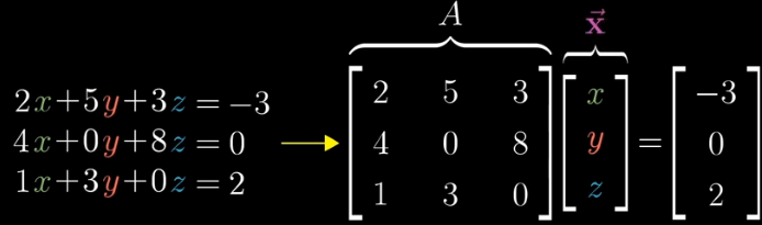
A linear transformation, for example, would take the 2D grid and perform any number of linear transformations on it - shrink, expand, twist, turn, etc and all of these are described by matrix transformations on top of our basis vectors
If is a transformation, and is a vector you want to find, such that when you transform you get to our desired output
So knowing this, if you have our output and a Transformation , you could hypothetically find the Inverse , which should give us our desired vector

This is useful because it allows us to understand how different transformations affect our vector space. Having a matrix and a vector , you can express the linear transformation as , where is the output vector. Alongside that, you can also consider the inverse transformation, which would allow us to map the output vector back to the input vector . In the grand scheme of things in the real world, the matrix represents linear combinations of weights and our output vector is our weighted sum of inputs / output. In graphics, ML, analytics, etc you use the matrix as a weight representation constantly, and it's just a way to transform our input vectors
Tracking the transformation of the basis vectors also allows us to track the output of any other vector in our system. If our basis is and , and a random starting vector is , you can express it in terms of our basis as . Therefore, if you apply the transformation to this space, you just have to track the effects on and , and then apply those effects to the starting vector.
There's a way to ultimately tell what a matrix transformation is doing to space by looking at the determinant of the matrix, which helps to understand how much area or volume is being scaled by the transformation. Formally the determinant calculation is a bit more complex, but the intuition is that it gives you a scalar value that represents how much the transformation scales areas (in 2D) or volumes (in 3D). A determinant of 1 means the area/volume is preserved, greater than 1 means it's expanded, and less than 1 means it's contracted. A determinant of 0 indicates that the transformation collapses the space into a lower dimension (e.g., a plane to a line). Having a non-zero determinant is crucial for ensuring that the transformation is invertible, meaning you can reverse the transformation and recover the original vectors (because no information is lost)
At the end of the day matrices are just transformations of space, that's IT!. Formally, a Linear Combination is defined as:
- Such that when multiplied by corresponding scalars
- you get to , where the are scalars
From the above, if you add them together , you can see that the output point is a linear combination of the input vectors
Therefore, a square matrix with a determinant allows us to solve a system of equations, to define a linear combination, and ultimately to find transformations that bring us from one point (usually the origin) to another fixed point via dimensional traversals
Span
The span of a set of vectors is the set of all points obtainable by linear combinations of the original vectors
- They define all of the points dimensionally you can "get to" from our basis vectors
- The particular span of all of the columns of is known as the Column Space or range of
- The basis vectors of are the vectors that span the column space of
- In 3D our basis vectors are where are the standard basis vectors representing , , and respectively
- Basis vectors are just the "unit vectors" which you can multiply, combine, and use to get to points in 3D space - any point in 3D cube can be reached uniquely by altering these 3 unit vectors
- If one of these was missing, say , our Z axis, then the Column Space of that set is 2D and we'd never be able to go up or down the Z axis - we'd be stuck in 2D!
- This point comes up repeatedly as "column space must be equal to ", but when stated this way it's less intuitive
Unique solutions also require Linear Independence, which means that no vector (column) in the basis vectors can be written as a linear combination of the others - if that were the case then one of our vectors could be removed without changing the span, which would contradict the definition of a basis
- For the linear system , having a unique solution (for a given ) requires that the columns of be linearly independent (i.e. full column rank)
- In the square case , linear independence of the columns is equivalent to , which makes invertible and guarantees a unique solution for every
- In a tall rectangular case , if the columns are independent and lies in the column space, then the solution is unique. If is outside the column space, there’s no solution
So how does this help us?
- Determining whether has a solution involves checking if is in the span of the columns of
- In order for to have a solution for all values of , it must be the case that the column space of is equal to (the space of all possible output vectors)
- Intuitively, this just means you need enough "directions" in our column space to reach any point in
- If one of the "directions" or dimensions in is unreachable because one of our basis vectors is missing or linearly dependent, then you can never reach that dimension
- In order for to have a solution for all values of , it must be the case that the column space of is equal to (the space of all possible output vectors)
Rank
The Rank of a matrix is a number, it's the dimension of the column space of the matrix - meaning how many dimensions does the output of the transformation span
- If the output of a transformation is a single point, you say the Rank is 0
- When the output of a transformation is a line, you say the Rank is 1
- If all output vectors land in 2D plane, the Rank is 2
- Therefore, Rank can be thought of as the number of dimensions in the output of the Transformation
- matrix with means nothing has collapsed, but matrix with the same Rank means something / some group of vectors or points has collapsed
Determinant
Determinant is based on Transformations, and can therefore be extended to matrices
Determinants help us to quantify how much Transformations scale unit areas of a metric space - meaning in a 2 dimensional space with and unit vectors, meaning a 1x1 = 1 area, if our Transformation turns that into a 2x3 area then our determinant would be 6
Determinants for 3 dimensional spaces would correspond to Volume of a cube, whereas 2 dimensional would be on flat area
Determinants also have signs for when there is an orientation flip, and a determinant of 0 would correspond to reduction of dimensions - meaning 2d down to 1d or single point
Given a matrix:
The determinant of is:
They are similar to integrals in that they both measure a form of "volume" - in the case of determinants, it's the volume of the parallelepiped formed by the column vectors of the matrix. Ultimately they just allow us to tell how much the transformation represented by the matrix "stretches" or "compresses" space.
Solutions to Linear Systems
Now that there's definitions in place, discussing solutions to Linear Systems makes more sense
For the examples below assume there's an input vector , a transformation , and an output vector as usual
Intuitively, having a solution means our metric space should have both and - if they're both in the metric space there must be a way to connect them through the transformation
The columns of span a certain subspace of (the column space), and they can be viewed as the images of the basis vectors that underlie the domain of the linear mapping (transformation). Therefore, only vectors inside of that reachable subscape can be "hit"
Determining whether or not has a solution involves checking if is in the span of the columns of - this is intuitive because it means that can be expressed as a linear combination of the columns of , which is necessary for there to exist some such that , if the was "living in another dimension" than then there would be no way to connect to it from
Really hitting on the points above because they're all interconnected
Taking for all values of , it must be the case that the column space of is equal to (the space of all possible output vectors). If any point in is not in the column space of , then there is no way to reach it from , and it's also a potential that we cannot reach - Intuitively, this just means you need enough "directions" in our column space to reach any point in . Immediately, this means that must have at least columns to be able to span - it could have more, and that would mean that the potential vectors we use would need to "sqush" down to a lower dimensional space. An example of this would be if we're working in 3D space, but our transformation only outputs 2D points - this would mean that our column space is a 2D plane in 3D space.
Another, clearer example, would be a matrix - in this the target is in , but the column space of can only span a 2D plane in that 3D space. Therefore, the only we can reach is one that lies in that 2D plane traced out by the column space of . Any that lies outside of that plane is unreachable, and therefore there is no solution for those
Intuitively now, having more columns than rows (i.e., more variables than equations) means that the system is underdetermined, and there may be infinitely many solutions or no solution at all, depending on whether lies in the column space of . It basically means there's "extra dimensions" in the input space that can be adjusted without affecting the output, leading to multiple possible vectors that map to the same
Conversely, having fewer columns than rows (more equations than variables) means the system is overdetermined, which can lead to no solution or a unique solution if the equations are consistent and independent. This is similar to the matrix example above, where the output space is larger than the input space, leading to potential unreachable outputs, so there are still some solutions we can find but there will most likely be unfindable ones
Invertibility Final Notes
Point 1: At the end of the day the column space of must be equal to for there to be a solution for every possible , and actually the condition is necessary and sufficient - meaning if the column space of is equal to , then there is a solution for every possible , and if there is a solution for every possible , then the column space of must be equal to
Point 2: For the matrix to have an inverse, we additionally need to ensure that has at most one solution for each in its column space. This requires that the columns of has at most columns. Otherwise, there's more than one way to parameterize each solution, leading to infinitely many solutions for some
Points 1 and 2 together means the matrix must be square () and have full rank () to ensure that has exactly one solution for every possible in . This is equivalent to saying that is invertible, which allows us to uniquely map each input vector to a distinct output vector , and vice versa
If the matrix isn't square there's other ways to solve it, but it won't be done via matrix inversion analytically
Altogether now: For a system of linear equations, and an output , there's either:
- No solution
- One exact solution
- There's one solution of if and only if is invertible, which corresponds to:
-
- If is a square matrix and then it's columns span all of
- If then it's columns do not span all of and there's none, or infinite, solutions
- (full rank)
- Columns of are linearly independent
- Columns of span all of
-
- All of the above imply each other, and intuitively mean that the transformation represented by is bijective (one-to-one and onto), allowing us to uniquely map each input vector to a distinct output vector , and vice versa
- There's one solution of if and only if is invertible, which corresponds to:
- Infinite solutions
- You can't have more than one but less than infinite - The idea: If you have one solution, you can always add a multiple of the null space to it to get another solution, thus creating infinitely many solutions.
- If both and are solutions, then is also a solution for any scalar
- The above solution has infinitely many solutions because you can choose any value for
- You can't have more than one but less than infinite - The idea: If you have one solution, you can always add a multiple of the null space to it to get another solution, thus creating infinitely many solutions.
Special Matrices
- Diagonal Matrix: A matrix where all off-diagonal elements are zero. It's written as where is a vector holding the scalar entries that represent the diagonal. It is represented as:
- These matrices are useful because multiplying them by a vector simply scales each component of by the corresponding diagonal entry which is computationally efficient
- The inverse is also computationally efficient to compute, as long as none of the diagonal entries are zero - it's simply the reciprocal of each diagonal entry
- Symmetric Matrix: A square matrix that is equal to its transpose, i.e., . This means that the elements are mirrored across the main diagonal:
- These often come about from functions of two arguments where the order of the arguments doesn't matter, such as distance metrics or covariance matrices
- Orthogonal Matrix: A square matrix whose columns (and rows) are orthonormal vectors. This means that , where is the identity matrix
- Orthogonal vectors have a dot product of zero, meaning they are perpendicular to each other in the vector space
- Orthonormal vectors are orthogonal vectors that also have a norm (length) of 1
- The inverse of an orthogonal matrix is simply its transpose:
- Geometrically, orthogonal matrices represent rotations and reflections in space without scaling
Eigenvalues, Eigenvectors, and Eigendecomposition
Eigenvalues and Eigenvectors are a weird subset of linear algebra that suck at first but are useful once understood
Mathematical objects are better understood by breaking them down into more fundamental components, and then studying those components and their similarities. Breaking down integers into prime factors, functions into Taylor series, and distributions into mean and variances is all examples of this
Eigenvalues and Eigenvectors are one such way of breaking down matrices (linear transformations) into more fundamental components
An Eigenvector of a square matrix is a non-zero vector such that multiplication with alters only the values of
- in this case the is the Eigenvalue corresponding to the Eigenvector
If is an Eigenvector of , then so is any rescaled vector , and moreover has the same Eigenvalue
Why does that matter? Intuitively it means that is a direction in space that is invariant under the transformation represented by - it only gets scaled by , not rotated or otherwise changed. They are useful methods for describing "concrete" bricks that make up a matrix transformation
If a matrix has linearly independent Eigenvectors with corresponding Eigenvalues , then these Eigenvectors can form a basis for . We can concatenate these Eigenvectors into a matrix where each column is an Eigenvector: And we can create a diagonal matrix with the corresponding Eigenvalues on the diagonal
Eigendecomposition is the process of decomposing a matrix into its eigenvalues and eigenvectors. For a square matrix , if it can be decomposed, it can be expressed as:
Constructing matrices with specific eigenvalues and eigenvectors enables us to stretch space in desired directions. The flip side is also true - decomposing a matrix into it's eigenvalues and eigenvectors allows for analyzing properties of the matrix
Every real symmetric matrix can bedecomposed into an expression using only real-valued eigenvectors and eigenvalues - this is known as the Spectral Theorem. This is particularly useful in many applications, such as Principal Component Analysis (PCA) in machine learning, where we analyze the covariance matrix of data to find the directions of maximum variance (the principal components), which are given by the eigenvectors of the covariance matrix
The solution above may not be unique because any two eigenvectors could share the same eigenvalue, so any set of orthogonal vectors lying in their span are also eigenvectors with that eigenvalue - this is known as the Eigenspace corresponding to that eigenvalue. The dimension of the eigenspace is called the geometric multiplicity of the eigenvalue
Singular Value Decomposition (SVD)
Singular Value Decomposition (SVD) is a technique in linear algebra that generalizes the concept of eigendecomposition to non-square matrices. SVD provides a way to factorize a matrix into singular vectors and singular values. Every real matrix of size can be decomposed using SVD, but not necessarily into eigenvalues and eigenvectors unless it is square and symmetric
In eigendecomposition: (which looks very similar to SVD calc below)
If is an matrix, and is real or complex, then SVD decomposes into three matrices: , , and , such that: Where:
- is an orthogonal matrix whose columns are the left singular vectors of
- is an diagonal matrix with non-negative real numbers on the diagonal, known as the singular values of
- is an orthogonal matrix whose columns are the right singular vectors of
The elements along are the singular values of , which are always non-negative and are typically arranged in descending order
The columns of are the left singular vectors of , and the columns of are the right singular vectors of . These singular vectors form orthonormal bases for the column space and row space of , respectively
Intuitively, SVD is used to show rotation / reflection with and , and scaling with . This helps show how much each independent direction is stretched or squeezed, and can quickly reveal rank and numeric stability in a linear transformation. Allows for a deeper understanding of the underlying structure of the data before doing anything crazy
Altogether, SVD provides a way to analyze and manipulate matrices, with applications in areas such as data compression, noise reduction, and latent semantic analysis. It's used to partially generalize matrix inversion to non-square matrices like in Moore-Penrose pseudoinverse
Moore-Penrose Pseudoinverse
The Moore-Penrose pseudoinverse is a generalization of the matrix inverse for non-square matrices. It's useful when has more rows than columns (i.e., ) or more columns than rows (i.e., ). It is denoted as and can be computed using the SVD of :
- Compute the SVD of :
- Form the pseudoinverse by taking the reciprocal of the non-zero singular values in and transposing the matrices:
Where is obtained by taking the reciprocal of each non-zero singular value in and transposing the resulting matrix.
Why is this useful?
- It provides a least-squares solution to linear systems that may not have a unique solution
- It can be used for dimensionality reduction and data compression
- It is widely used in machine learning algorithms, particularly in linear regression and support vector machines
At the end of the day it's an extension of the concept of matrix inversion to a broader class of problems, making it a solution that's more realistic to use in day-to-day problems versus "perfectly square, nice" matrices
Trace Operator
The trace operator is the sum of all the diagonal entries of a matrix - it's a pretty simple operation: The trace is written inline as .
It's used in a few different algorithms, but nothing much more to discuss
Example: Principal Component Analysis (PCA)
Principal Component Analysis (PCA) is a dimensionality reduction technique that is widely used in machine learning and statistics. It transforms the data into a new coordinate system, where the greatest variances lie on the first coordinates (called principal components)
These principal components, ideally, allow us to combine our original inputs into less dimensions while retaining a majority of the variance - if we can go from 100 dimensions down to 2 or 3, we can visualize our data much more easily while still capturing the important patterns, and if we keep 95% of the variance in the 2 dimensions it helps ensure that we're not losing critical information about the data
Suppose there's a collection of points - , where each is a point in . The goal of PCA is to find a new set of axes (the principal components) that maximize the variance of the projected data. A typical example involves performing "lossy" compression over these points, which means reducing the number of dimensions while preserving as much information as possible. A way of doing this would be encoding these points in a lower-dimensional version - for each in we find a corresponding vector in , where
Ideally there's an encoding function such that , and a corresponding decoding function such that
PCA is actually defined by the choice of that decoding function - typically a linear function of the form , where is a weight matrix and is a bias vector
To make the above concept easier, is usually chosen so that it's columns are orthogonal to each other (to ensure that the principal components are uncorrelated), and to have unit norm (to ensure unique solutions)
Achieving PCA
To turn the above concepts into a practical algorithm, PCA must:
- Figure out how to generate the optimal code point for each input point , and so ideally we can minimize the distance
Which will simplify to
And after some more simplification and multiplying things out, it comes out to
Which is solved via vector calculus and simple optimization techniques like gradient descent - specifically, we can use the fact that the gradient of a quadratic function is linear, allowing us to iteratively update our code points until convergence
Everything ends up coming down to
So the optimal function is given by the projection of onto the subspace spanned by the columns of
How to find this projection? It's known that minimizing the distance between inputs and reconstructions is ideal output
If we stack all of our input vectors into a matrix , where each row is an input vector, we can express the optimization problem in terms of this matrix
Therefore, is the matrix of all code points, where there are rows of features
Create a covariance matrix
Eigendecomposition is then applied to this covariance matrix to find its eigenvalues and eigenvectors. The eigenvectors represent the directions of maximum variance in the data, while the eigenvalues indicate the amount of variance captured by each eigenvector - after this decomposition, we will have our optimal code points for
The covariance matrix is sort of a "magical solution thing" that just solves most of the core optimization problem - so dissecting that is crucial for understanding PCA. The covariance matrix ties together span, rank, eigenvalues, eigenvectors, SVD, projections, and pretty much every other topic from above:
- Intuition: Multiplying the data matrix by its transpose and scaling by gives us the covariance matrix which intuitively just measures how much the different dimensions of the data vary together
- How do eigenvectors intuitively relay this information? As you multiply a vector by itself , you're essentially measuring how much each dimension of the data aligns with every other dimension - the directions where this alignment is strongest correspond to the eigenvectors of the covariance matrix
- The vectors underlying the covariance matrix that simply shrink or expand, but do not rotate
- Let's say you have to project data onto a single 1D vector . The optimal projection can be found by minimizing the distance between the original data points and their projections onto
- What do you choose as ? The optimal choice is the vector corresponding that "captures" the most variance in your dataset
- Covariance is a measure of how much two random variables change together
- The covariance matrix captures this relationship for all pairs of dimensions in the data, so it will compare each row to every other row
- The vectors underlying the covariance matrix that simply shrink or expand, but do not rotate
- Comparing every data point to each other shows how they vary together, and so underlying eigenvectors of this covariance relationship represent the directions along which the data is most spread out
- The actual covariance linear transformation will form an ellipses
- This ellipses represents the distribution of data in feature space
- In picture below, and are the principal components

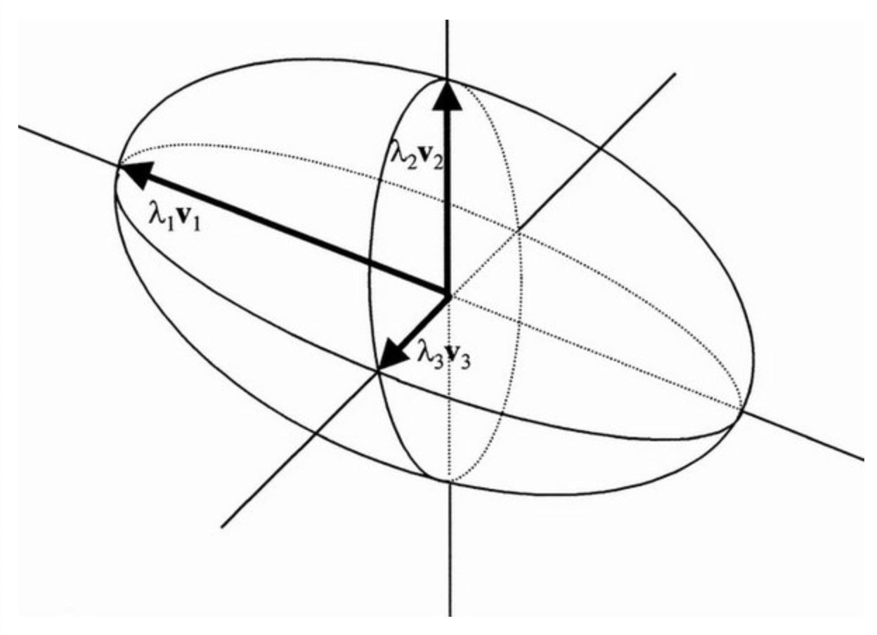
- How do eigenvectors intuitively relay this information? As you multiply a vector by itself , you're essentially measuring how much each dimension of the data aligns with every other dimension - the directions where this alignment is strongest correspond to the eigenvectors of the covariance matrix
- Rank: The rank of the covariance matrix is equal to the number of non-zero eigenvalues, which corresponds to the number of dimensions in the data that have variance
- Span / Column Space: The top principal components (eigenvectors) form an orthonormal basis for the -dimensional subspace capturing the most variance
- Their span is where the low-rank reconstruction lives
- Eigenvalues and vectors: Eigenvalues represent the amount of variance captured by each principal component (eigenvector), and the larger the value the more variance is captured by that component
- Determinant: The determinant of the covariance matrix provides a measure of the volume of the space spanned by the principal components, with a larger determinant indicating a more "spread out" distribution of the data
- I.e. it's how much variance is "covered" by PCA
So after a lot of algebra, the optimization problem is solved using eigendecomposition - specifically, we look for the eigenvectors of the covariance matrix of the data, which are the directions of maximum variance. The principal components are then given by the top eigenvectors, where is the desired dimensionality of the reduced space